Updated June 9, 2023
Excel Consolidation (Table of Contents)
Consolidate Data in Excel
Consolidate in Excel combines the data of more than 2 workbooks in the Data menu tab under the Data tools section with the name Consolidate. For this, we must have the same data type in different workbooks. Although different data sets will also work, there will not be proper alignment in consolidated data. Choose any mathematical function which we want to execute at last. Then select all the data using references from all the workbooks and click OK. This will combine the selected tables with the execution of the chosen mathematical function at the end.
How to Consolidate Data in Multiple Worksheets?
Let’s understand how to consolidate data in multiple worksheets with a few examples.
Example #1 – Consolidate Data in the Same Workbook
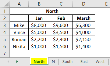
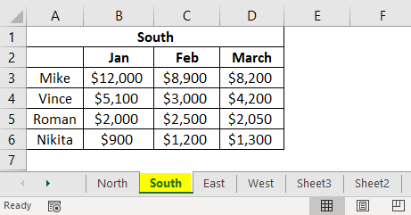
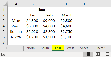
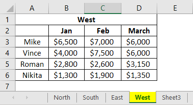
Let’s say we have a worksheet with sales data with four worksheets marked as per their region as North, South, East, and West. Now we want to consolidate the data into one place rather than in a sheet within the same workbook. There is a fifth sheet named consolidated file.
This example will show the consolidated sales for all the regions. First, here are the sample data files. You can see the worksheet names and the last consolidated file we must work on here.
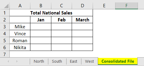
This is our template in the “consolidated file” sheet, and now we will start consolidating data from the worksheets.
We will now click on cell B3.
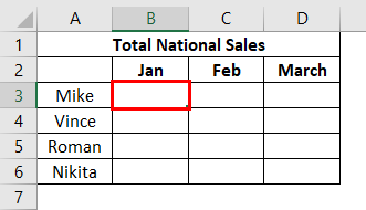
We want the “Consolidate” function to insert the data from other sheets. As we can see above, cell B3 is selected, and now we will move up to the Data tab in Excel Ribbon and go to Consolidate.
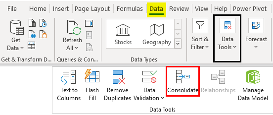
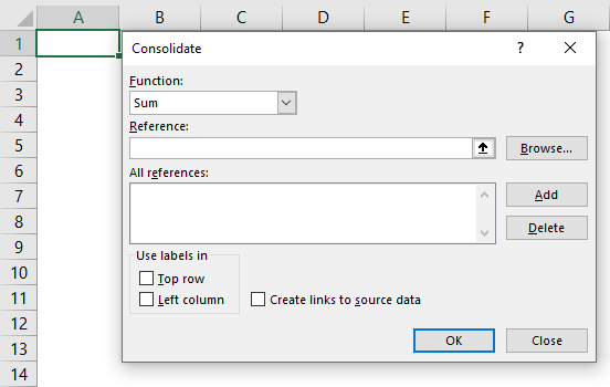
Once we click on Consolidate, the below window will appear:
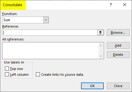
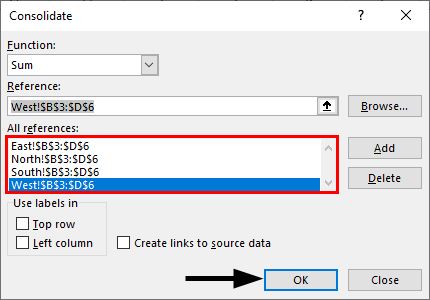
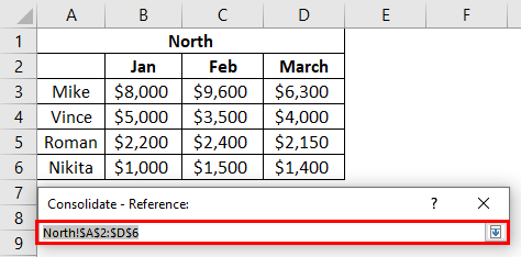
The first thing we look at is the “Function” dropdown which shows many arithmetic functions like sum, count, max, average, etc. Since we want a sum of sales, we will select “Sum” in the dropdown. Now, we will go to the reference tab to add a reference to our data from different worksheets. We will then go to our first sheet containing North’s sales data. We only have to select sales data and not heading and rows. This is shown below.
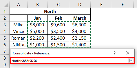
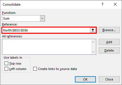
The reference is shown in the “Reference” box like this.
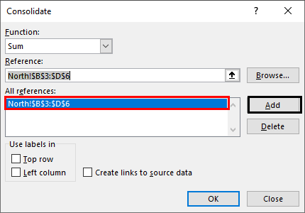
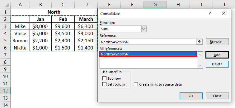
Click “Add,” and the reference will be added in the “All Reference “box.
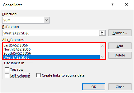
Similarly, we will now add a reference from all other sheets like North, South, East, and West. Once we have finished adding the references, click “OK”.
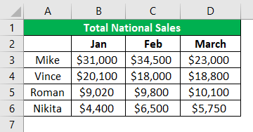
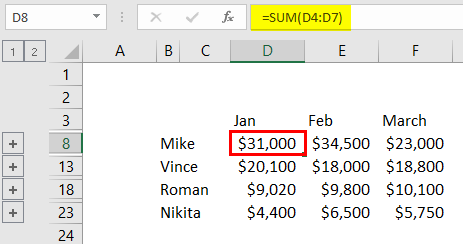
Now we have consolidated data for sales for the executives month-wise, at a national level.
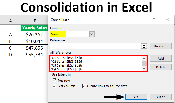
Example #2 – Consolidate Yearly Sales Product Wise
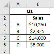
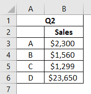
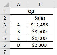
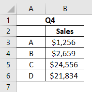
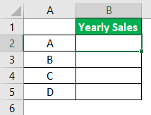
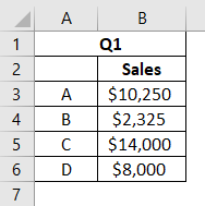
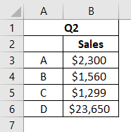
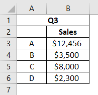
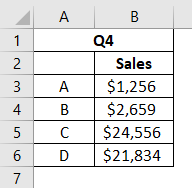
In this, we have quarter wise sales for products A, B, C, and D, and we want consolidated yearly sales product-wise.
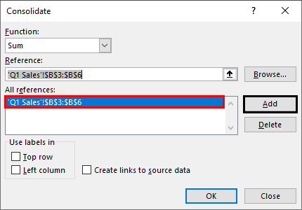
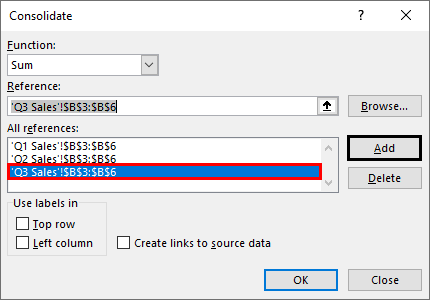
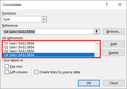
We will now go to the reference tab to add references to our data from different worksheets. Here we have data in four sheets; the first sheet with sales data for Q1 next has data for Q2, followed by data for Q3 and Q4. We will go to our first sheet, which contains the sales data for Q1. We will select the data as shown below.
Now, we will go to the Data tab and click Consolidate, and the below window will appear.
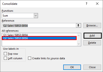
We will click “Add,” and the reference will be added in the “All reference “box.
We will click “Add,” and the reference will be added in the “All reference “box.
We will click “Add,” and the reference will be added in the “All reference “box.
Below is our template for the consolidated datasheet. We will now select cell B2 to get the total sales data from other sheets.
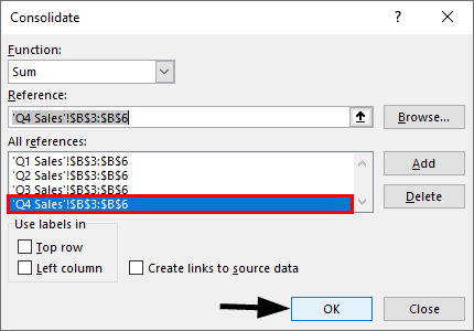
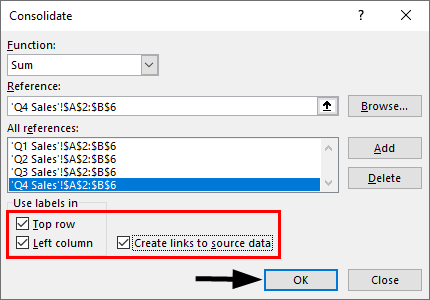
We will select the “Sum “function from the drop-down. Likewise, we will add references from sheets Q2, Q3, and Q4. It will appear like this. All the references from all the sheets are now added. Click “OK”
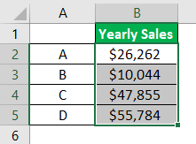
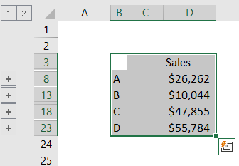
We now have our consolidated yearly sales data with the sum totals for each product.
Taking our previous sample data, we will do the consolidation below. It is also possible to insert the consolidated table into a blank worksheet instead of creating a template table.
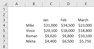
We don’t have a template for the consolidation table, and we want to get consolidated data in a blank worksheet with row and column labels. We will add a new worksheet; in our case, it is a “Consolidated file”.
Like before, we will go to the Data tab<Consolidation. Select “Sum” from the drop-down list.
We will now select the reference from our datasheets. And start this with the “North” sheet and will then proceed with “South”, “East”, and “West” sheets. We will select the data below, including row and column labels.
We will then add the reference in the “All references” box:
Now add all the references in the same way from all the datasheets.
We will now check the “Top Row” and “Left Column” and press OK.
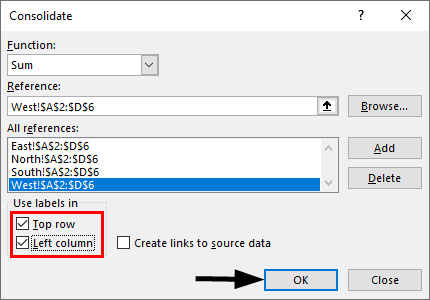
We now see consolidated sales data with row and column labels.
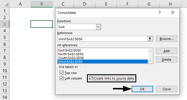
If you want to update the consolidated data when the individual sheet gets updated, click on the box “Create Links to create data”. If you’re going to update data manually, don’t check the box and click OK.
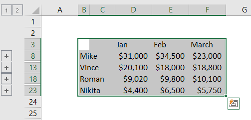
The cells in the consolidated table now contain the sum formula, as shown below. This makes it dynamic in nature.
This is a dynamic consolidation table.
Example #3 – Consolidating Data From Different Workbooks
Suppose we have data in different workbooks and want to consolidate it into a single workbook. This gives us great flexibility and ease. We can do this as well.
We have quarterly sales data for various products, say A, B, C, and D, in different workbooks, as shown below.
Once all the workbooks are open, we will go to a new workbook and click on cell B3. Add the references from all the worksheets below.
We have consolidated data from all the workbooks into a new workbook.
Moreover, any changes in the data in any workbook will also get updated in the new consolidated data workbook.
So we have learned how to use the consolidation function in Excel with the help of examples. It is useful in merging or collecting data into one sheet from different worksheets or workbooks.
Things to Remember About Consolidation in Excel
- Be careful in selecting reference data when checking the boxes for “Top Row” and “Left Column”. You must then select the complete data, including the row and column labels.
- When you are consolidating data of dynamic nature from different worksheets and workbooks, check the “create links to source data”, which will automatically update the changes in the data if done.
Recommended Articles
This is a guide to Consolidation in Excel. Here we discuss How to Consolidate Data in Multiple worksheets, practical examples, and a downloadable Excel template. You can also go through our other related articles –
