Updated June 6, 2023
Excel HYPERLINK Formula
Hyperlink formula in excel is used to create a shortcut path to quickly jump to any sheet, website or folder. We all have seen this even of many websites where a word highlighted in blue fonts consists of a hyperlink that would take us to some other location if we click on it. The same function works in excel, in the name of Hyperlink.
Syntax:
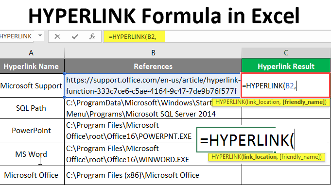
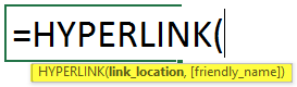
HYPERLINK () – It will return a shortcut of the given workbook references or URL, which used to be in blue color and underlined. There is a two-parameter – (link_location and [friendly_name]).
An argument in the Hyperlink Function:
- link_location: The file or workbook reference is a mandatory parameter that needs to be opened.
- friendly_name: It is an optional parameter, the name of the hyperlink created by the function. By default, it will take Link location as the friendly name.
How to Use HYPERLINK Formula in Excel?
HYPERLINK Formula in Excel is straightforward. Let’s understand how to use the HYPERLINK Formula in Excel with some examples.
Example #1 – Basic Hyperlink Function
Let’s look at how to Use the basic Hyperlink Function for inside workbook references in Excel. A user with the name of the hyperlink name gives some references. He wants to create a hyperlink for all the references within the same workbook.
Let’s see how the Hyperlink Function can solve this problem. Open MS Excel, Go to Sheet1, where the user wants to create a hyperlink for all references.
Create one column header for the Hyperlink Result to show the function result in the C column.
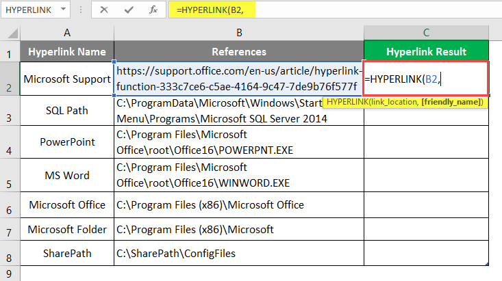
Click on cell C2 and apply Hyperlink Formula.
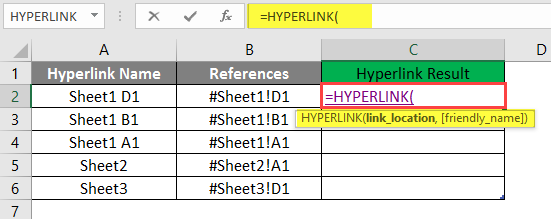
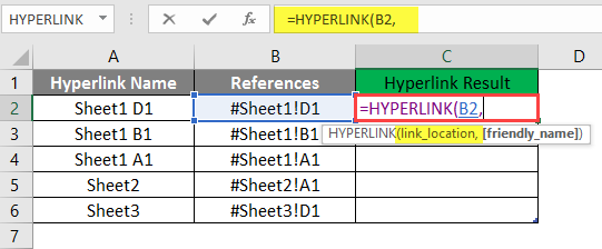
Now it will ask for the link location, select the reference given in B Column, and select cell C2.
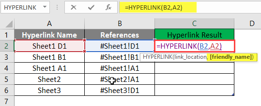
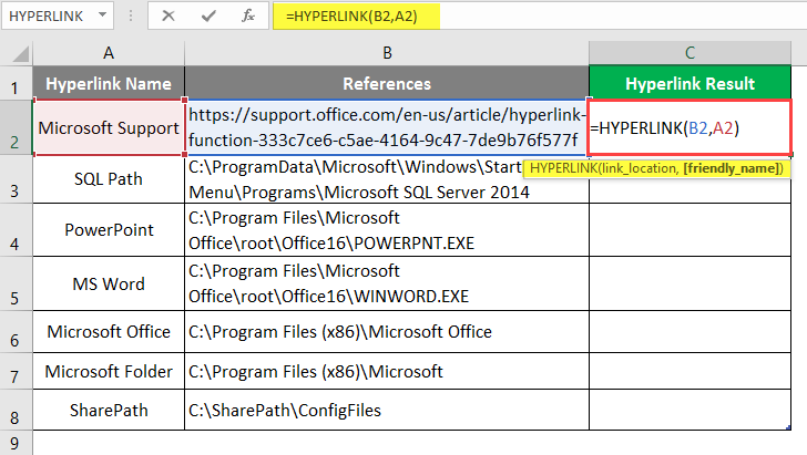
It will then ask for a familiar name, which the user wants to give as the Hyperlink Name, available in the A2 cell and written in the C2 cell.
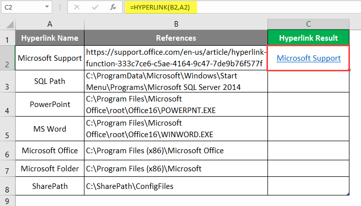
Press the Enter key.
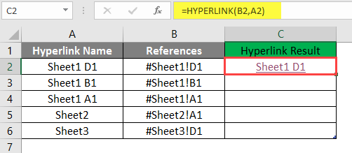
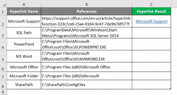
Drag the formula to the other C column cell to find the Hyperlink Result.
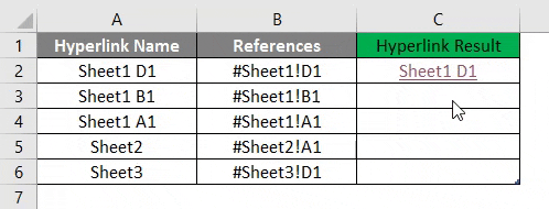
Summary of Example 1:
As the user wants to create HYPERLINK for all given references, the same the user achieved by the Hyperlink Function. Which is available in the D column as the Hyperlink result.
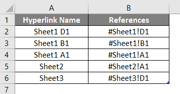
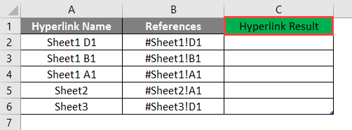
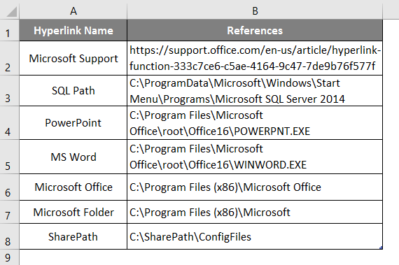
Example #2 – Outside Workbook References
Let’s learn how to use the Hyperlink function for outside workbook references like URLs and folder paths in Excel. There are some references given by a user with the name of the hyperlink name, which is either URLs or folder paths. He wants to create a hyperlink for all the references outside the workbook.
Let’s see how the Hyperlink Function can solve this problem. Open MS Excel, Go to Sheet2, where the user wants to create a hyperlink for all references.
Create one column header for the Hyperlink Result to show the function result in column C.
Click on the C2 cell and apply Hyperlink Formula.
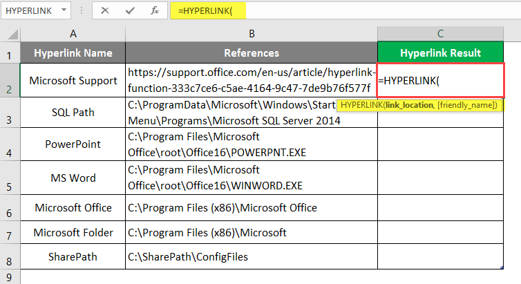
Now it will ask for the link location, select the reference given in Column B, and select cell B2.
Now it will ask for a familiar name, which the user wants to give as the hyperlink name.
Press the Enter key.
Drag the same function to the other cell of column C to find out the HYPERLINK result.
Summary of Example 2:
As the user wants to create HYPERLINK for all given references, the same the user achieved by the Hyperlink Function. Which is available in column D as the Hyperlink result.
Example #3 – Sending E-Mail
Let’s find out how to use the Hyperlink Function for sending an E-Mail to someone in Excel.
An MS Health company wants to create a hyperlink to send welcome mail by clicking on the hyperlink in Excel. They have one format for the welcome mail, which they send to every new employee who joins MS Health Pvt Ltd. In E-Mail content, they have Email-Address, Subject, Mail Body, and Company Signature.
Let’s see how the Hyperlink Function can solve this problem. Open MS Excel, Go to Sheet 3, where the user wants to create a hyperlink for all references.
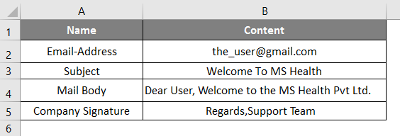
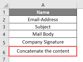
Create one column header for the Concatenate mail content in the A6 cell.
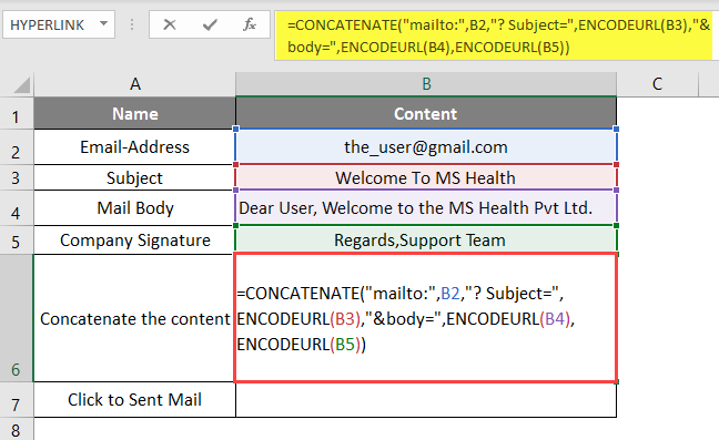
Click on cell B6 and apply to CONCATENATE Function to join all mail content like email-id, subject, mail body, and signature.
Note:
- “Mailto:” command to send the mail;
- “?subject=” Command to write the subject;
- “& body =” – Command to write the main body text;
Click on cell B7 and apply the Hyperlink Formula.
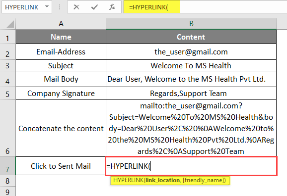
Now it will ask for the link location; select the reference in the B6 cell.
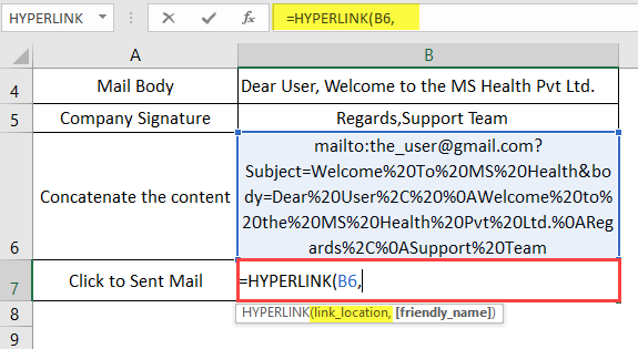
Now it will ask for a familiar name, which the user wants to give as the hyperlink name, available in cell A7 and cell B7.
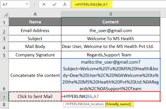
Press the Enter key. Now click on the hyperlink to find out the HYPERLINK result.
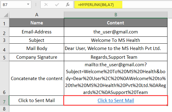
A Window will open, as shown below.
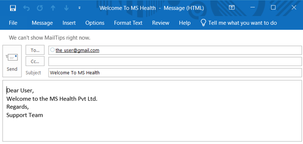
Summary of Example 3: As the MS Health company wants to create a hyperlink to send a welcome e-mail by clicking on the hyperlink in Excel their format for the welcome mail, which they use to send every new employee who joins MS Health Pvt Ltd. Same implemented in the above example no 3.
Things to Remember
- The Hyperlink Function will return a hyperlink, a shortcut of the given workbook references or URL, which used to be underlined in blue colure.
- By default, it will take Link location as a familiar name.
- If a user wants to select all the hyperlinks without going to the link location, use the arrow key from the keyboard and select the hyperlink cells.
- There is some command to write mail content in Excel: “Mailto:” command to send mail; “?subject=” Command to write subject; “& body =” – the command to write the text.
Recommended Articles
This has been a guide to HYPERLINK Formula in Excel. Here we discuss How to use HYPERLINK Formula in Excel, practical examples, and a downloadable Excel template. You can also go through our other suggested articles –
