Updated April 25, 2023
Introduction to Logistic Regression in R
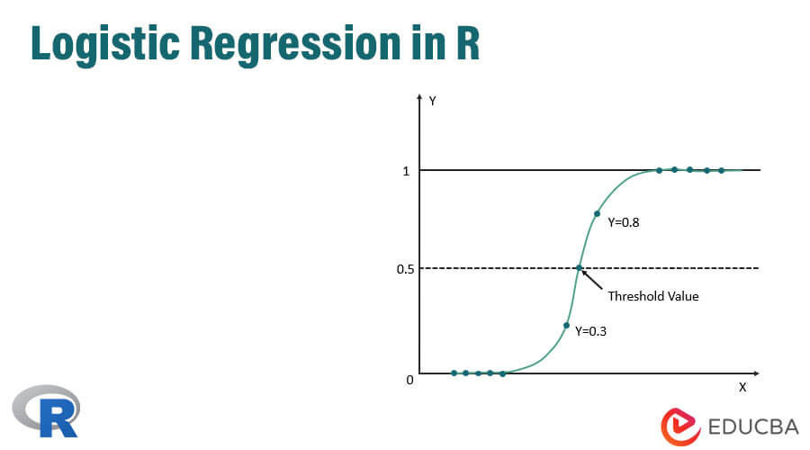
Logistic regression in R is defined as the binary classification problem in the field of statistic measuring. The difference between a dependent and independent variable with the guide of logistic function by estimating the different occurrence of the probabilities, i.e., it is used to predict the outcome of the independent variable (1 or 0 either yes/no) as it is an extension of a linear regression which is used to predict the continuous output variables.
How does Logistic Regression in R works?
Logistic regression is a technique used in the field of statistics measuring the difference between a dependent and independent variable with the guide of logistic function by estimating the different occurrence of probabilities. They can be either binomial (has yes or No outcome) or multinomial (Fair vs poor very poor). The probability values lie between 0 and 1, and the variable should be positive (<1).
It targets the dependent variable and has the following steps to follow:
- n- no. of fixed trials on a taken dataset.
- With two outcomes trial.
- The outcome of the probability should be independent of each other.
- The probability of success and failures must be the same at each trial.
In this, we are considering an example by taking the ISLR package, which provides various datasets for training. To fit the model, the generalized linear model function (glm) is used here. To build a logistic regression glm function is preferred and gets the details of them using a summary for analysis task.
Working Steps:
The working steps on logistic regression follow certain term elements like:
- Modeling the probability of doing probability estimation
- Prediction
- Initializing threshold value (High or Low specificity)
- Confusion matrix
- The plotting area under the curve(AUC)
Examples to Implement of Logistic Regression in R
Below are some example of Logistic Regression in R:
- data loading: Installing the ISLR package.
- require(ISLR)
- loading required package: ISLR
For this article, we are going to use a dataset ‘Weekly’ in RStudio. The dataset implies the summary details of the weekly stock from 1990 to 2010.
- require(ISLR)
- names(OJ)
Output:
[1] “Purchase” “WeekofPurchase”, “StoreID”, “PriceCH” [5] “PriceMM” “DiscCH” “DiscMM” “SpecialCH” [9] “SpecialMM” “LoyalCH” “SalePriceMM” “SalePriceCH” [13] “PriceDiff” “Store7” “PctDiscMM” “PctDiscCH” [17] ” ListPriceDiff” “STORE”str(OJ)
Shows 1070 Observations of 18 variables.
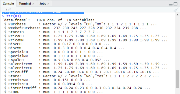
Our dataset has 1070 observations and 18 different variables. Here we have Special MM, And special CH has a dependent outcome. Let’s take a Special MM attribute to have a correct observation and an accuracy of 84 %.
table(OJ$SpecialMM)
0 1
897 173
Next, to find the probability
897/1070
[1] 0.8383178In the next step for a better sample Splitting the data set into training and testing data set is a goo
- library(caTools)
- set.seed(88)
- split=sample.split(OJ$SpecialMM, SplitRatio = 0.84)
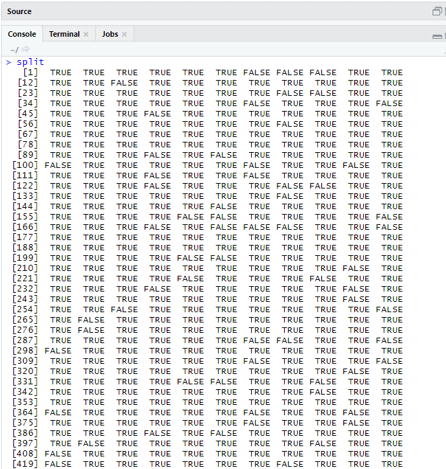
Considering qt has a training set and qs has test set sample data.
- qt=subset(OJ,split==TRUE)
- qs=subset(OJ,split==FALSE)
nrow(qt)
[1] 898nrow(qs)
[1] 172Therefore we have 898 Training set and 172 testing samples.
Next using Summary () gives the details of deviance and co-efficient tables for regression analysis.
- QualityLog=glm(SpecialMM~SalePriceMM+WeekofPurchase ,data=qt,family=binomial)
- summary(QualityLog)
Output:
| Call:
glm(formula = SpecialMM ~ SalePriceMM + WeekofPurchase, family = binomial, data = qt) Deviance Residuals: Min 1Q Median 3Q Max -1.2790 -0.4182 -0.3687 -0.2640 2.4284 Coefficients: Estimate Std. Error z value Pr(>|z|) (Intercept) 2.910774 1.616328 1.801 0.07173 . SalePriceMM -4.538464 0.405808 -11.184 < 2e-16 *** WeekofPurchase 0.015546 0.005831 2.666 0.00767 ** — Null deviance:794.01 on 897 degrees of freedom Residual deviance: 636.13 on 895 degrees of freedom AIC: 642.13 Number of Fisher Scoring iterations: 5 |
From the above analysis, it is said that the coefficients table gives positive values for WeekofPurchase, and they have at least two stars which imply they are the significant codes to the model.
Example #1 – Prediction Technique
Here we shall use the predict Train function in this R package and provide probabilities; we use an argument named type=response. First, let’s see the prediction applied to the training set (qt). The R predicts the outcome in the form of P(y=1|X) with the boundary probability of 0.5.
predictTrain = predict(QualityLog, type=”response”)
Summary results in median, mean, and min, max values.
summary(predictTrain) Execution gives
Min. 1st Qu.Median Mean 3rd Qu.Max.
0.02192 0.03342 0.07799 0.16147 0.25395 0.89038
tapply (predictTrain,qt$SpecialMM)
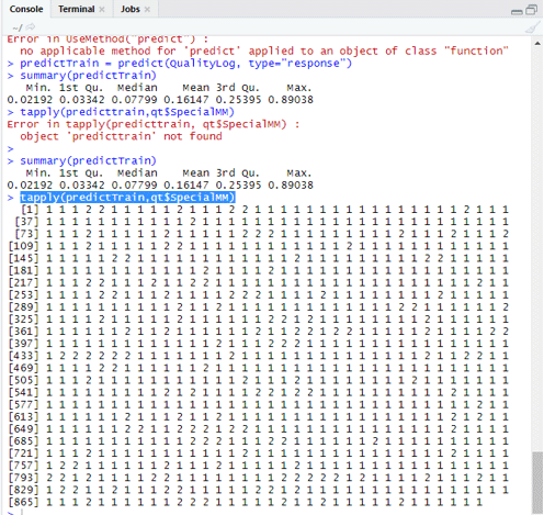
To compute the average for the true probabilities tapply() function is used.
tapply(predictTrain,qt$SpecialMM,mean)
0 1
0.1224444 0.3641334
Therefore, we find in the above statement that the possibility of true SpecialMM means value is0.34 and for true poor value is 0.12.
Example #2 – Calculating Threshold Value
if P is > T– prediction is poor Special MM
if P is <T– Prediction is good
Classification Matrix:
table(qt$SpecialMM,predictTrain >0.5)
FALSE TRUE
0 746 7
1 105 40
To compute Sensitivity and Specificity
40/145
[1] 0.2758621746/753
[1] 0.9907039Testing set Prediction
predictTest = predict(QualityLog, type = “response”, newdata = qs)
table(qs$SpecialMM,predictTest >= 0.3)
FALSE TRUE
0 130 14
1 10 18
table(qs$SpecialMM,predictTest >= 0.5)
FALSE TRUE
0 140 4
1 18 10
Calculating accuracy
150/172
[1] 0.872093There are 172 cases from which 144 are good, and 28 are poor.
Plotting ROC Curve: This is the last step by plotting the ROC curve for performance measurements. A good AUC value should be nearer to 1, not to 0.5. Checking with the probabilities 0.5, 0.7, 0.2 to predict how the threshold value increases and decreases. It is done by plotting threshold values simultaneously in the ROC curve. A good choice is picking, considering higher sensitivity.
Logistic Regression Techniques
Let’s see an implementation of logistic using R, as it makes it very easy to fit the model.
There are two types of techniques:
- Multinomial Logistic Regression
- Ordinal Logistic Regression
Former works with response variables when they have more than or equal two classes. later works when the order is significant.
Conclusion
Hence, we have learned the basic logic behind regression alongside we have implemented Logistic Regression on a particular dataset of R. A binomial or binary regression measures categorical values of binary responses and predictor variables. They play a vital role in analytics wherein industry experts are expecting to know the linear and logistic regression. They have their own challenges, and in the practical example, we have done the steps on data cleaning, pre-processing. Altogether we have seen how logistic regression solves a problem of categorical outcome in a simple and easy way.
Recommended Articles
This has been a guide to Logistic Regression in R. Here, we discuss the working, different techniques, and broad explanation on different methods used in Logistic Regression in R. You may also look at the following articles to learn more –
