Updated March 20, 2023
What is Linear Regression in R?
Linear Regression in R is an unsupervised machine learning algorithm. R language has a built-in function called lm() to evaluate and generate the linear regression model for analytics. The regression model in R signifies the relation between one variable known as the outcome of a continuous variable Y by using one or more predictor variables as X. It generates an equation of a straight line for the two-dimensional axis view for the data points. Based on the quality of the data set, the model in R generates better regression coefficients for the model accuracy. The model using R can be a good fit machine learning model for predicting the sales revenue of an organization for the next quarter for a particular product range.
Linear Regression in R can be categorized into two ways.
1. Simple Linear Regression
This is the regression where the output variable is a function of a single input variable. Representation of simple linear regression:
y = c0 + c1*x1
2. Multiple Linear Regression
This is the regression where the output variable is a function of a multiple-input variable.
y = c0 + c1*x1 + c2*x2
In both the above cases c0, c1, c2 are the coefficient’s which represents regression weights.
Linear Regression in R
R is a very powerful statistical tool. So let’s see how it can be performed in R and how its output values can be interpreted. Let’s prepare a dataset, to perform and understand regression in-depth now.
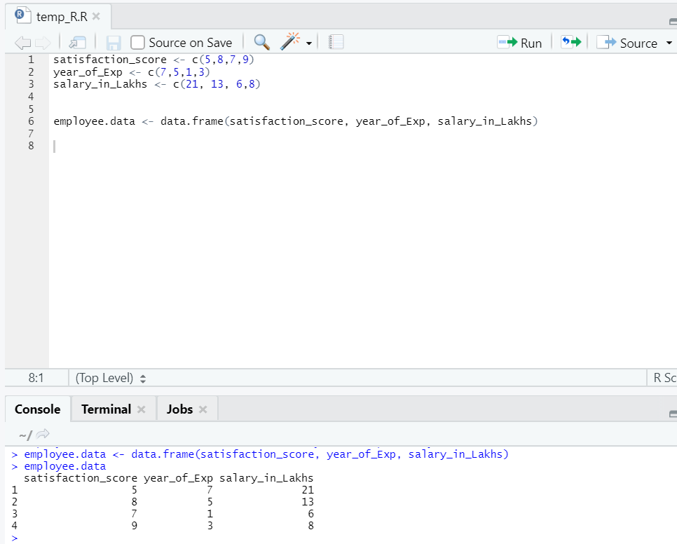
Now we have a dataset where “satisfaction_score” and “year_of_Exp” are the independent variable. “salary_in_lakhs” is the output variable.
Referring to the above dataset, the problem we want to address here through linear regression is:
Estimation of the salary of an employee, based on his year of experience and satisfaction score in his company.
R code:
model <- lm(salary_in_Lakhs ~ satisfaction_score + year_of_Exp, data = employee.data)

summary(model)
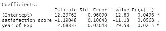
The output of the above code will be:
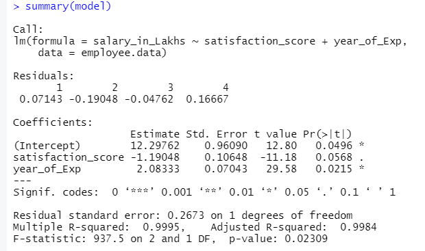
The formula of Regression becomes
Y = 12.29-1.19*satisfaction_score+2.08×2*year_of_Exp
In case one has multiple inputs to the model.
Then R code can be:
model <- lm(salary_in_Lakhs ~ ., data = employee.data)
However, if someone wants to select a variable out of multiple input variables, there are multiple techniques like “Backward Elimination”, “Forward Selection”, etc. that are available to do that as well.
Interpretation of Linear Regression in R
Below are some interpretations in r, which are as follows:
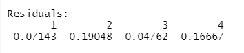
1. Residuals
This refers to the difference between the actual response and the predicted response of the model. So for every point, there will be one actual response and one predicted response. Hence residuals will be as many as observations are. In our case, we have four observations, hence four residuals.
2. Coefficients
Going further, we will find the coefficients section, which depicts the intercept and slope. If one wants to predict an employee’s salary based on his experience and satisfaction score, one needs to develop a model formula based on slope and intercept. This formula will help you in predicting salary. The intercept and slope help an analyst to come up with the best model that suits datapoints aptly.
Slope: Depicts the steepness of the line.
Intercept: The location where the line cuts the axis.
Let’s understand how formula formation is done based on slope and intercept.
Say intercept is 3, and the slope is 5.
So, the formula is y = 3+5x. This means if x is increased by a unit, y gets increased by 5.
a. Coefficient – Estimate: In this, the intercept denotes the average value of the output variable when all input becomes zero. So, in our case, salary in lakhs will be 12.29Lakhs as average considering satisfaction score and experience comes zero. Here slope represents the change in the output variable with a unit change in the input variable.
b. Coefficient – Standard Error: The standard error is the estimation of error we can get when calculating the difference between our response variable’s actual and predicted value. In turn, this tells about the confidence for relating input and output variables.
c. Coefficient – t value: This value gives the confidence to reject the null hypothesis. The greater the value away from zero, the bigger the confidence to reject the null hypothesis and establishing the relationship between output and input variable. In our case value is away from zero as well.
d. Coefficient – Pr(>t): This acronym basically depicts the p-value. The closer it is to zero, the easier we can to reject the null hypothesis. The line we see in our case, this value is near to zero; we can say there exists a relationship between salary package, satisfaction score and year of experience.
Multiple R-squared, Adjusted R-squared
R-squared is a very important statistical measure in understanding how close the data has fitted into the model. Hence in our case, how well our model that is linear regression represents the dataset.
R-squared value always lies between 0 and 1. Formula is:
![]()
The closer the value to 1, the better the model describes the datasets and their variance.
However, when more than one input variable comes into the picture, the adjusted R squared value is preferred.
F-Statistic
It’s a strong measure to determine the relationship between input and response variables. The larger the value than 1, the higher is the confidence in the relationship between the input and output variable.
In our case, it’s “937.5”, which is relatively larger considering the size of the data. Hence the rejection of the null hypothesis gets easier.
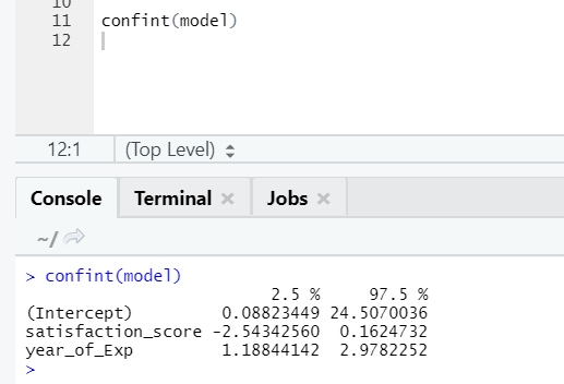
If someone wants to see the confidence interval for the model’s coefficients, here is the way to do it:-
Visualization of Regression
R Code:
plot(salary_in_Lakhs ~ satisfaction_score + year_of_Exp, data = employee.data)

abline(model)
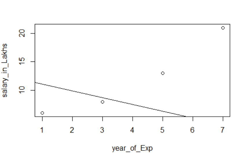
It’s always better to gather more and more points before fitting to a model.
Conclusion
Linear regression is simple, easy to fit, easy to understand, yet a very powerful model. We saw how linear regression could be performed on R. We also tried interpreting the results, which can help you in the optimization of the model. Once one gets comfortable with simple linear regression, one should try multiple linear regression. Along with this, as linear regression is sensitive to outliers, one must look into it before jumping into the fitting to linear regression directly.
Recommended Articles
This is a guide to Linear Regression in R. Here, we have discussed what is Linear Regression in R? categorization, Visualization, and interpretation of R. You can also go through our other suggested articles to learn more –
