Updated August 22, 2023
Excel KPI Dashboard (Table of Contents)
Introduction to KPI Dashboard in Excel
Key Performance Indicator, a.k.a. KPI dashboard, is a versatile dashboards that can be used occasionally and then as per business requirements. Most of the time, it is a graphical representation of different business processes that have progressed along with some already set (predefined) measures for goal achievement. The KPI dashboard provides the nicest view of KPIs and their comparison over other KPIs. This article will show some KPI dashboards and how to make such from scratch. Those are nothing but visual measures, which allows you to quickly check whether the current business values are going as expected or not in the easiest way (just looking at the graph) without checking a bunch of data. Thow
How to Create KPI Dashboard in Excel?
Let’s understand how to create the KPI Dashboard in Excel with some examples.
Example #1 – KPI Dashboard in Excel using PowerPivot
PowerPivot is not new to Excel users. You can develop many fancy reports using this tool from Excel without taking any help from IT people. Moreover, KPI is a new addition to PowerPivot, allowing you to check the performance in a jiffy even though you have millions of rows. We will see in this example how to create a simple KPI using PowerPivot.
First thing first, you have to enable Power Pivot in your Excel.
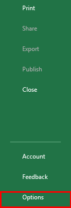
Step 1: Open an Excel file. Click on the File tab on the uppermost ribbon. Go to Options.
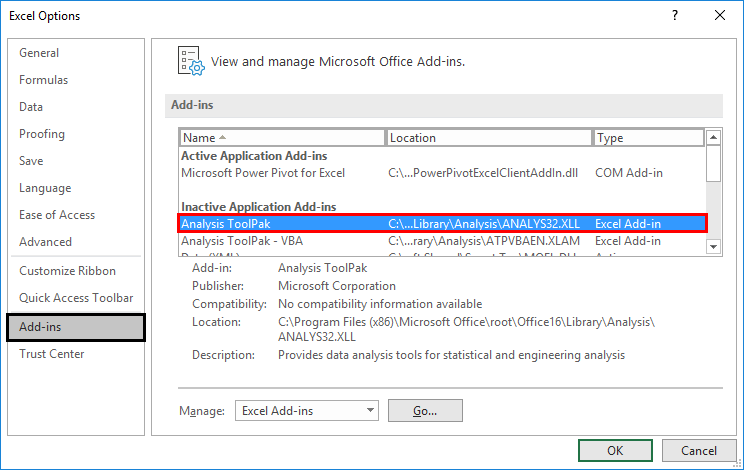
Step 2: Under Options > Click on Add-ins. You’ll be able to see the screen as shown below.
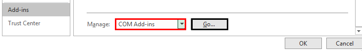
Step 3: Select COM Add-ins under the Manage section dropdown and click the Go button.
Step 4: When you hit the Go button, the COM Add-ins dialog box will pop up. Select Microsoft Power Pivot for Excel from the list of add-ins and click OK.
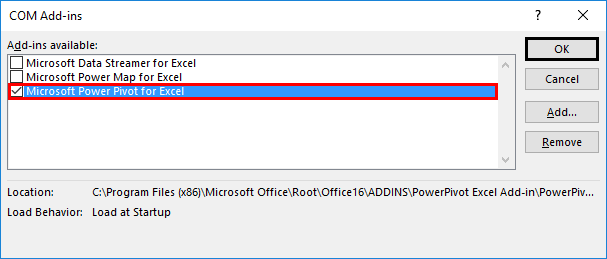
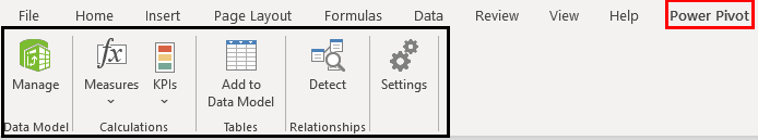
After enabling this PowerPivot add-in, you should see the PowerPivot option tab on the topmost panel ribbon in your Excel.
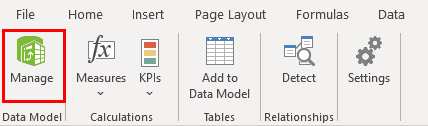
Step 5: Now, the actual work begins. Under the PowerPivot tab in your Excel file, click on Manage.
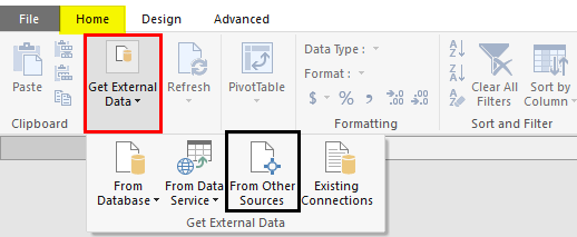
Step 6: It should open a new tab named Power Pivot for Excel. There are different ways to import data under PowerPivot. Click the Database tab to add data from SQL Server, Access. However, if you have an Excel file or text file, or some data files other than SQL and Access, please click on From Other Sources tab.
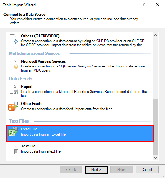
Step 7: A new window named Table Import Wizard will pop up once you click on the “From Other Sources” tab. There are many options from where you can import the data to PowerPivot. Select the Excel file, then click the Next button to proceed.
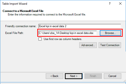
Step 8: Browse the path where your Excel data file is stored and click the Next button to finish the Import.
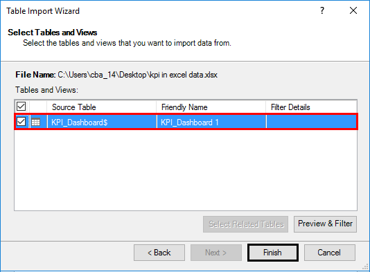
Step 9: Click the Finish button once the data table is loaded into PowerPivot.
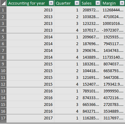
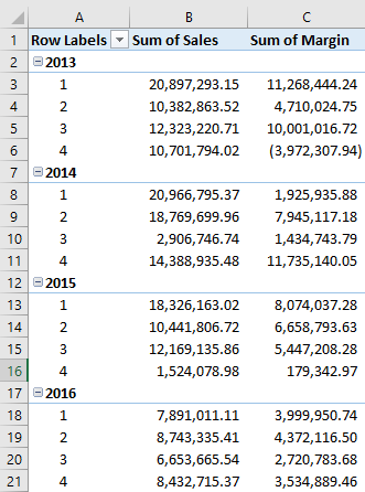
Step 10: You can see the data below after a successful import.
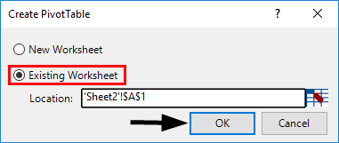
Step 11: To create a KPI report, we need to slice and dice our data under the pivot table. Click on the Pivot Table tab under PowerPivot. Once you click it, a new window named Create PivotTable will appear in which you have to select the data from PowerPivot, and it asks you whether you want a pivot table under a new sheet or on the same sheet. I will prefer to go with the same sheet and then will provide the range on which the pivot table should be added. Click OK once done.
Step 12: Select the data under rows, columns, and values, as shown below.
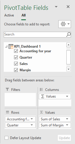
Here we have selected data in the following order:
Rows: Accounting Date Year & Quarter
Values: Sum of Sales & Margin
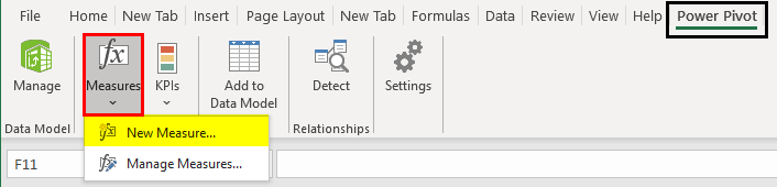
Step 13: We will add a calculated column in the pivot. Select Measures under the Excel sheet. Click on New Measures.
A new window called Measure will pop up. It will allow you to formulate and add a measure under your pivot table.
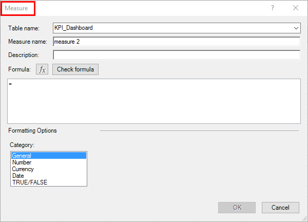
Step 14: Under” Measure name:“, add a name for your measure (For e.g., Margin%). If you want to add a description for the same, you can also add it under the Description section. Under the Formula section, add the formula =[Sum of Margin]/[Sum of Sales] as shown below. It will calculate the Margin% for you. See the screenshot below.
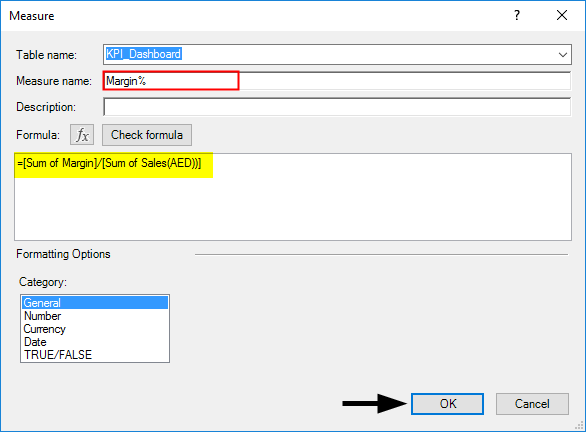
Here, we have created a new calculated column named Margin%, formulated as the ratio of two columns, Sum of Margin and Sum of Sales. Once you are done with this step, click on the OK button, and you will see a new calculated column named Margin% under the pivot table.
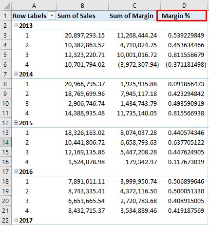
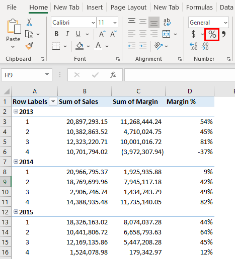
Step 15: Select the entire column, Margin %, and convert it to % using number formatting.
Step 16: Our data is ready for KPIs to be added. Click on the KPIs tab, as shown in the figure. Select the New KPI option.
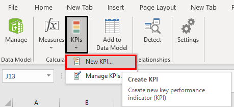
A KPI window will pop up, as shown below. It has some by default values, which we are going to change.
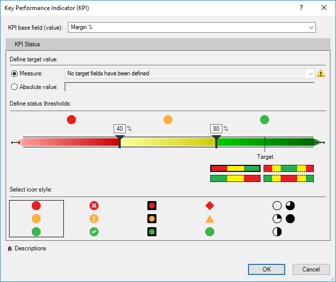
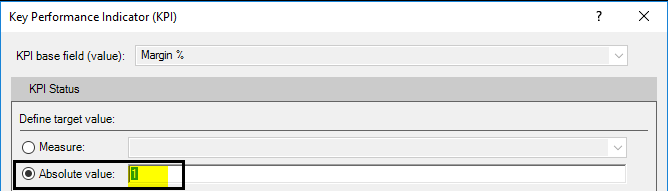
Step 17: In this window, define an Absolute Value for the target as 1. We are doing this because we don’t have any other target values/measures defined separately to compare with actual values of Margin %.
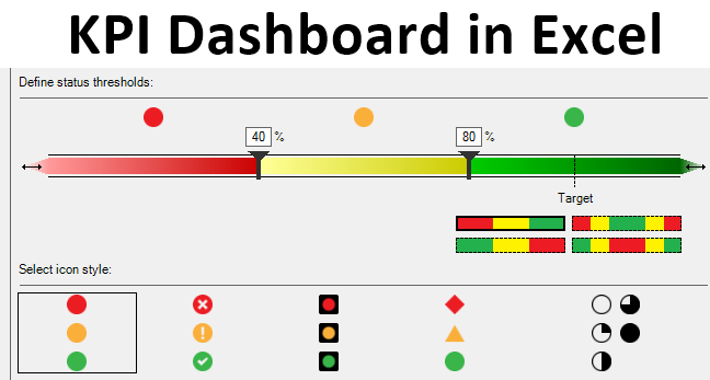
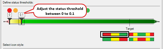
Step 18: In this step, define the Status Threshold value. It is defined in decimal format. If 40% will be given as 0.40, change the Status Threshold values as shown in the screenshot below.
Step 19: Now, we can also select icon style (These are the KPI Icons). I will opt out of the second style. As shown below.
![]()
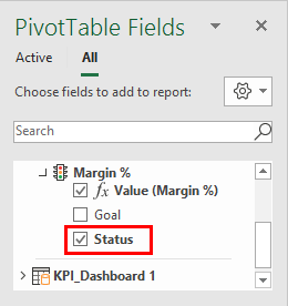
Step 20: Click OK once you set the KPI parameters and customization.
![]()
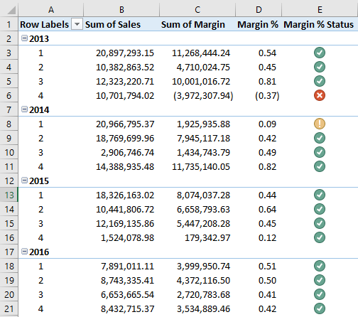
Tada, your KPI Dashboard is ready and will look as shown in the screenshot below.
Things to Remember About KPI Dashboard in Excel
- You always need to assign data to PowerPivot to be used to create the KPI Dashboard.
- Every time, you must add a pivot once the data is imported into PowerPivot for KPI Dashboard creation.
Recommended Articles
This is a guide to KPI Dashboard in Excel. Here we discuss How to create KPI Dashboard in Excel, practical examples, and a downloadable Excel template. You can also go through our other suggested articles –
