Updated April 28, 2023
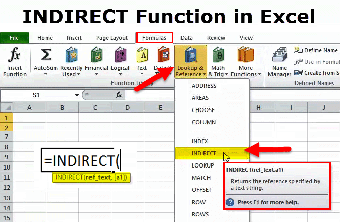
Excel INDIRECT Function
Indirect function in Excel returns a valid reference from the selected text string or in other words which we can say it converts a text string into valid references. This looks a little complex but when we see the syntax of the indirect function we will notice, it just requires Reference Text from any cell as a mandatory field.
INDIRECT Formula in Excel:
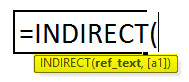
An INDIRECT function consists of two arguments. One is Ref_Text which is a mandatory argument, and the second one is [a1].
- Ref_Text: It refers to a cell containing either An A1-style reference or An R1C1-Style Reference, A name defined by the name/formula, or A reference to a cell in text form. This argument can reference another workbook.
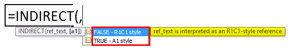
- [a1]: It is an optional argument. This argument consists of two logical values, TRUE or FALSE. Whatever value we got in Ref_Text shows as A1-Style Reference if it is TRUE and shows as R1C1 Style Reference if it is FALSE.
How to Use the INDIRECT Function in Excel?
An INDIRECT function in Excel is very simple and easy to use. Let us now see how to use the INDIRECT Function in Excel with the help of some examples.
Example #1 – Named Ranges
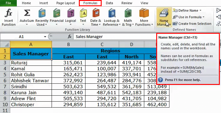
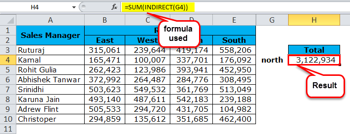
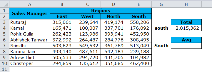
The below table shows the sales amount of different sales managers across 4 regions. In cell H4, we need to get the region’s total mentioned in cell G4.
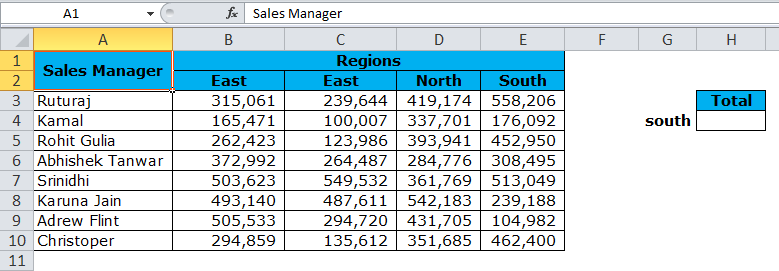
A combination of INDIRECT & Named Ranges is invaluable in this context. Named Range will define the range of cells in a single name.
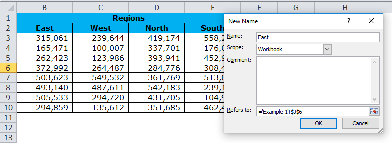
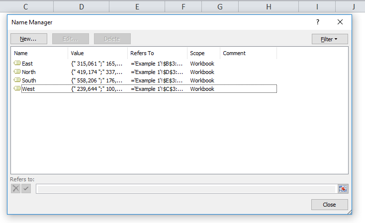
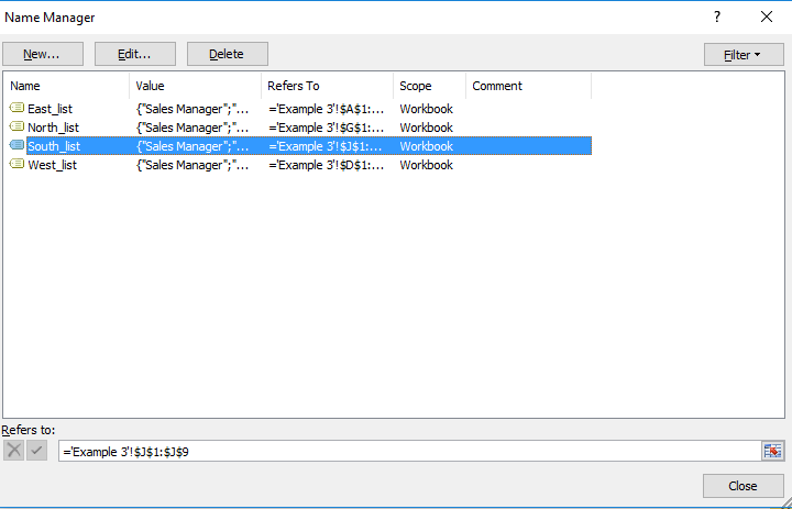
Step 1: Create a named range for each region. Go to the Formula tab and then click on Name Manager.
A New Name dialog box appears. Give the name East.
Step 2: Now apply the INDIRECT and SUM functions to get the total in cell H4.
Example #2 – Average Function
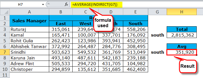
Use the previous sales amount data of different sales managers across 4 regions. In cell H7, we need to get the average total of the region, which is mentioned in cell G7.
Now apply the INDIRECT and AVERAGE functions to get the total in cell H4.
Example #3 – Return the last cell value
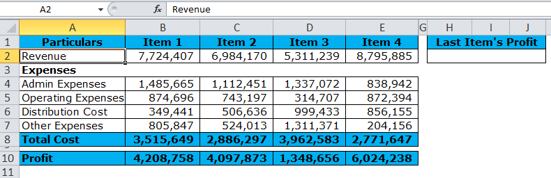
With the help of the below data, we need to find the last item’s Profit value. In cell H2, the last item’s profit.
This example will look into the R1C1 style reference with INDIRECT to return the last cell value. Here we used the COUNTA function to get the last column number.
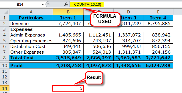
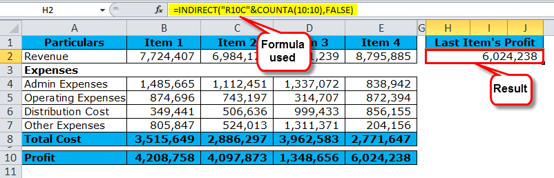
We have concatenated R10 (Row 10) with C10 using the COUNTA function in the above formula. COUNTA will return the value 5 (last column number). A combination of these will give “R10C5”, i.e. Indirect will value Row 10 and Column 5.
The FALSE part of the argument will request an R1C1 style of the cell reference.
As the Item numbers keep increasing, this function will always give the last item’s profit value.
Example #4 – INDIRECT + Named Range + VLookup
A combination of Indirect with Named Range & Vlookup will be a dynamic combination. It is necessary to include the example of Indirect with Vlookup.
The table below applies the VLOOKUP function in cell B15 to get the sales value based on cells B13 & B14.
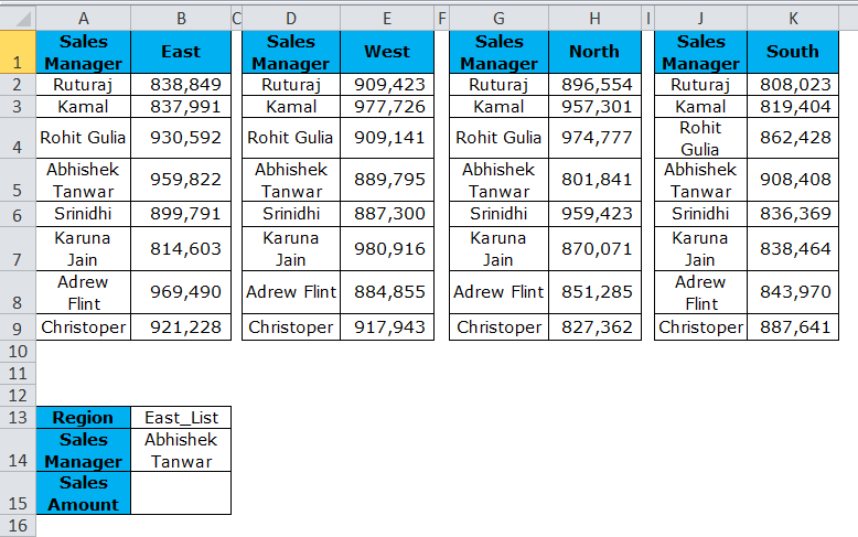
Steps involved before applying Vlookup.
- Create a dropdown list for both the region & sales manager list
- Create 4 named ranges (refer to example 1) for all 4 regions. Please note that apply named ranges, including the sales manager’s name.
- After the above two steps, apply the VLOOKUP function in cell B15.
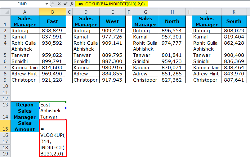
Since we have defined a range list with East_List, West_List, North_List, and South_List, what the INDIRECT function will do is it will give a reference to that particular region list. Therefore, Vlookup will consider that as a table range and give the respective sales manager the result.
From the drop-down list, change the play with different regions & different sales managers.
Example #5 – Refer to Worksheet with INDIRECT
An INDIRECT function can also retrieve the cell value from another worksheet. This example will explain this.
- An indirect Sheet is a sheet we are entering a formula.
- The summary Sheet is the sheet where data is there.
- In the Indirect Sheet, enter the formula in cell C2.
- You need to give a reference to cell B7 in the Summary Sheet.
Below images will show different sheets in a single window.
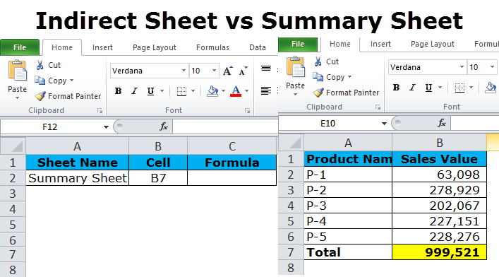
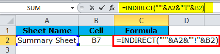
Here we have concatenated the Summary Sheet in cell A2 of the Indirect Sheet & referenced the B7 cell from the Summary Sheet in the Indirect Sheet.
Things to Remember
- The reference must be valid; otherwise, the function will return a #REF error.
- When referring to the other workbook, the respective workbook should be in an open mode to get the results.
- Generally, an INDIRECT function will return an A1 style reference by default.
- When using [a1] reference as FALSE, we need to put 0 and 1 for TRUE.
- In R1C1 style reference, you can use formulas like COUNTA to dynamically give a reference to the row or column. If the data increases, it will be a dynamic function and need not change now and then.
Recommended Articles
This has been a guide to INDIRECT. Here we discuss the INDIRECT Formula and how to use the INDIRECT function, along with practical examples and downloadable Excel templates. You may also have a look at these other lookup and reference functions in Excel-
