Updated March 22, 2023
Introduction to Graphs in R
Graphs in R language is a preferred feature which is used to create various types of graphs and charts for visualizations. R language supports a rich set of packages and functionalities to create the graphs using the input data set for data analytics. The most commonly used graphs in the R language are scattered plots, box plots, line graphs, pie charts, histograms, and bar charts. R graphs support both two dimensional and three-dimensional plots for exploratory data analysis.There are R function like plot(), barplot(), pie() are used to develop graphs in R language. R package like ggplot2 supports advance graphs functionalities.
Types of Graphs in R
A variety of graphs is available in R, and the use is solely governed by the context. However, exploratory analysis requires the use of certain graphs in R, which must be used for analyzing data. We shall now look into some of such important graphs in R.
For the demonstration of various charts, we are going to use the “trees” dataset available in the base installation. More details about the dataset can be discovered using? trees command in R.
1. Histogram
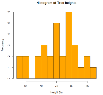
A histogram is a graphical tool that works on a single variable. Numerous variable values are grouped into bins, and a number of values termed as the frequency are calculated. This calculation is then used to plot frequency bars in the respective beans. The height of a bar is represented by frequency.
In R, we can employ the hist() function as shown below, to generate the histogram. A simple histogram of tree heights is shown below.
Code:
hist(trees$Height, breaks = 10, col = "orange", main = "Histogram of Tree heights", xlab = "Height Bin")
Output:
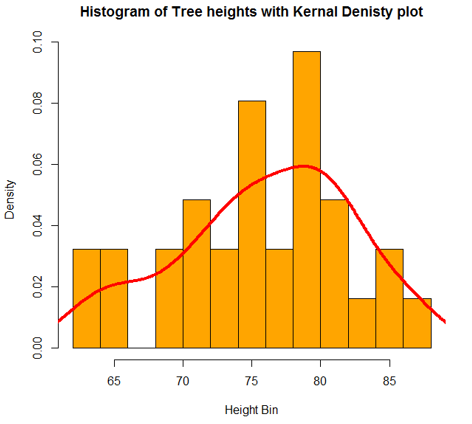
To understand the trend of frequency, we can add a density plot over the above histogram. This offers more insights into data distribution, skewness, kurtosis, etc. The following code does this, and the output is shown following the code.
Code:
hist(trees$Height, breaks = 10, col = "orange",

+ main = "Histogram of Tree heights with Kernal Denisty plot",

+ xlab = "Height Bin", prob = TRUE)
Output:
2. Scatterplot
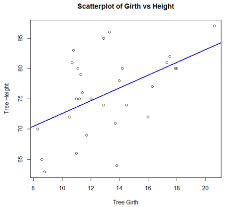
This plot is a simple chart type, but a very crucial one having tremendous significance. The chart gives the idea about a correlation amongst variables and is a handy tool in an exploratory analysis.
The following code generates a simple Scatterplot chart. We have added a trend line to it, to understand the trend, the data represents.
Code:
attach(trees)

plot(Girth, Height, main = "Scatterplot of Girth vs Height", xlab = "Tree Girth", ylab = "Tree Height")

abline(lm(Height ~ Girth), col = "blue", lwd = 2)
Output:
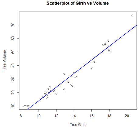
The chart created by the following code shows that there exists a good correlation between tree girth and tree volume.
Code:
plot(Girth, Volume, main = "Scatterplot of Girth vs Volume", xlab = "Tree Girth", ylab = "Tree Volume")

abline(lm(Volume ~ Girth), col = "blue", lwd = 2)
Output:
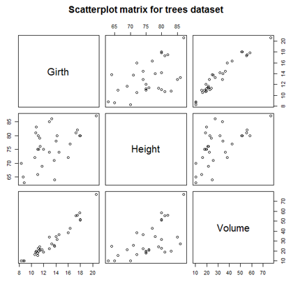
Scatterplot Matrices
R allows us to compare multiple variables at a time because of it uses scatterplot matrices. Implementing the visualization is quite simple, and can be achieved using pairs() function as shown below.
Code:
pairs(trees, main = "Scatterplot matrix for trees dataset")
Output:
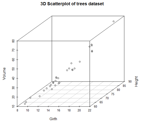
Scatterplot3d
They make visualization possible in three dimensions which can help to understand the relationship between multiple variables. So, to make scatterplots available in 3d, firstly scatterplot3d package must be installed. So, the following code generates a 3d graph as shown below the code.
Code:
library(scatterplot3d)

attach(trees)

scatterplot3d(Girth, Height, Volume, main = "3D Scatterplot of trees dataset")
Output:
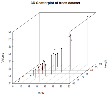
We can add dropping-lines and colors, using the below code. Now, we can conveniently distinguish between different variables.
Code:
scatterplot3d(Girth, Height, Volume, pch = 20, highlight.3d = TRUE,

+ type = "h", main = "3D Scatterplot of trees dataset")
Output:
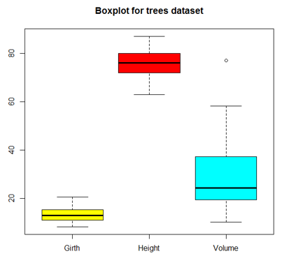
3. Boxplot
Boxplot is a way of visualizing data through boxes and whiskers. Firstly, variable values are sorted in ascending order and then the data is divided into quarters.
The box in the plot is the middle 50% of the data, known as IQR. The black line in the box represents the median.
Code:
boxplot(trees, col = c("yellow", "red", "cyan"), main = "Boxplot for trees dataset")
Output:
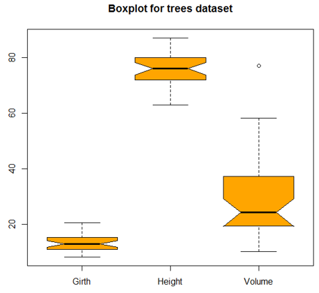
A variant of the boxplot, with notches, is as shown below.
Code:
boxplot(trees, col = "orange", notch = TRUE, main = "Boxplot for trees dataset")
Output:
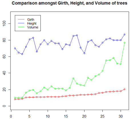
4. Line Chart
Line charts are useful when comparing multiple variables. They help us relationship between multiple variables in a single plot. In the following illustration, we will try to understand the trend of three tree features. So, as shown in the below code, initially, and the line chart for Girth is plotted using plot() function. Then line charts for Height and Volume are plotted on the same plot using lines() function.
The “ylim” parameter in plot() function has been, to accommodate all three line charts properly. Having legend is important here, as it helps understand which line represents which variable. In the legend “lty = 1:1” parameter means that we have the same line type for all variables, and “cex” represents the size of the points.
Code:
plot(Girth, type = "o", col = "red", ylab = "", ylim = c(0, 110),

+ main = "Comparison amongst Girth, Height, and Volume of trees")

lines(Height, type = "o", col = "blue")

lines(Volume, type = "o", col = "green")

legend(1, 110, legend = c("Girth", "Height", "Volume"),

+ col = c("red", "blue", "green"), lty = 1:1, cex = 0.9)
Output:
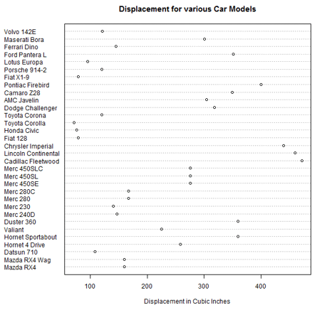
5. Dot plot
This visualization tool is useful if we want to compare multiple categories against a certain measure. For the below illustration, mtcars dataset has been used. The dotchart() function plots displacement for various car models as below.
Code:
attach(mtcars)

dotchart(disp, labels = row.names(mtcars), cex = 0.75,

+ main = "Displacement for various Car Models", xlab = "Displacement in Cubic Inches")
Output:
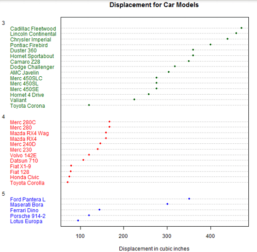
So, now we will sort the dataset on displacement values, and then plot them by different gears using dotchart() function.
Code:
m <- mtcars[order(mtcars$disp),]
m$gear <- factor(m$gear)

m$color[m$gear == 3] <- "darkgreen"

m$color[m$gear == 4] <- "red"

m$color[m$gear == 5] <- "blue"

dotchart(m$disp, labels = row.names(m), groups = m$gear, color = m$color, cex = 0.75, pch = 20,

+ main = "Displacement for Car Models", xlab = "Displacement in cubic inches")
Output:
Conclusion
Analytics in a true sense is leveraged only through visualizations. R, as a statistical tool, offers strong visualization capabilities. So, the numerous options associated with charts is what makes them special. Each of the charts has its own application and the chart should be studied prior to applying it to a problem.
Recommended Articles
This is a guide to Graphs in R. Here we discuss the introduction and types of graphs in R such as histogram, scatterplot, boxplot and much more along with examples and implementation. You may also look at the following articles to learn more –
