Updated August 10, 2023
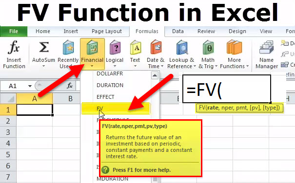
FV Function in Excel
FV function in Excel, where FV stands for future value, is used to calculate the future value of investment or loan amount forgiven, rate of interest, and fixed installment, which must be made at the start or end of the period or month.
It’s a type of Financial function. FV stands for ‘Future Value’ and calculates the future value of an investment based on a constant interest rate.
Syntax
Explanation
The FV formula in Excel has the following arguments:
- Rate: Interest rate per period.
- Nper: Total number of payment periods in an annuity.
- Pmt (Optional argument): The payment made each period.
- Note: It cannot change over the life of the annuity. Pmt contains only principal and interest but no other fees or taxes. If Pmt is omitted, you must include the PV argument.
- Pv (Optional argument): The present value, or the lump-sum amount that a series of future payments is worth.
- Note: If pv is omitted, it is assumed to be 0 (zero), and you must include the Pmt argument.
- Type (Optional argument): 0 or 1 indicates when payments are due. If the type is omitted, it is assumed to be 0.
- If payments are due
- 0 – At the end of the period
- or
- 1 – At the beginning of the period
How to Use the FV Function in Excel? (Examples)
Let us now see how to use the FV function in Excel with the help of some examples.
Example #1
In this FV in Excel example, if you deposit an amount of $1000.00 for 5 years at the rate of interest provided at 10%, then the future value that will be received at the end of the 5th year will be calculated in the following manner.
Opening Balance = OB
Deposit Balance= DB
Interest Rate = R
Closing Balance= CB
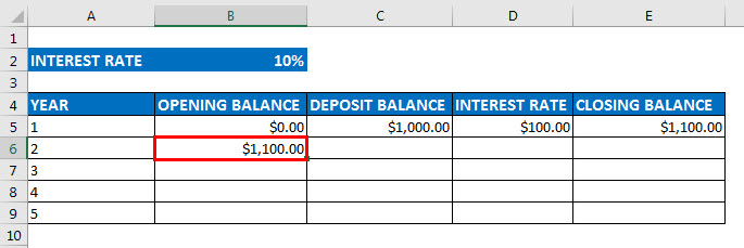
The opening balance at the beginning of the year (1st Year) will be nil, which is $0.
Now, let the amount deposited in the account is $1000.00.
So, the interest in 1st year at 10% will be
(OB + DB) *R
= (0+1000) *0.10 equals $100.00
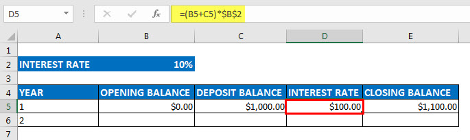
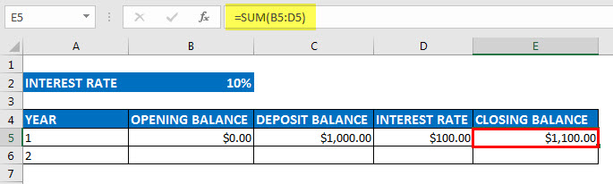
So, the closing balance of the 1st year will be
(OB+DB+IR)
= (0.00+1000.00+100.00) equals $1100.00
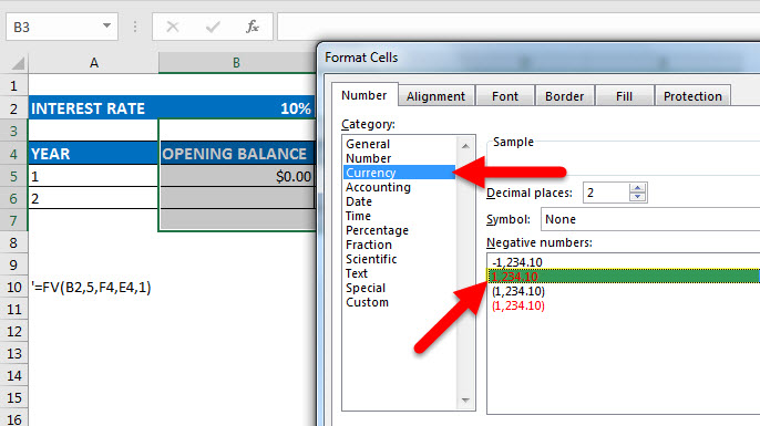
Prior to start, change the cells’ format to CURRENCY FORMAT with 2 decimal places for the columns from opening balance to closing balance.
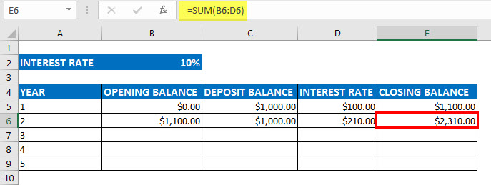
Year Opening Balance Deposit Balance Interest Rate Closing Balance
1 $0.00 $1,000.00 $100.00 $1,100.00
2 $1,100.00 $1,000.00 $210.00 $2,310.00
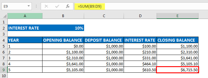
3 $2,310.00 $1,000.00 $331.00 $3,641.00
4 $3,641.00 $1,000.00 $464.10 $5,105.10
5 $5,105.10 $1,000.00 $610.51 $6,715.61
The deposited amount in the 3rd column remains the same throughout the 5 years.
In the 2nd column, we have the opening balance each year; in the first year, we have to start opening the balance with a nil account, which is the amount that will be $0.
Column four displays the interest payment for each year. An interest rate is 10% in the first year. So, the interest payment in 1st year will be the sum of the opening balance, deposited balance & interest value. Then, finally, the closing balance in the 5th column will be calculated as the sum of all the balances, the sum of the opening balance, the deposited amount, and the interest amount. So, in 1st year we received an interesting weight of $100.00.
So, $1100.00 will be the opening balance for the next year that is the second year.
Again, we are receiving a deposit of the amount of $1000.00 in the second year, and similarly, the interest rate & closing balance is calculated in the same manner as the first one.
A similar calculation is done for all five years, So, at the end of the 5th year computing it the same way, we get the final future value amount which is $6,715.50
Now, this can be directly calculated using the FV function in Excel, by the following method, under the formula toolbar select financially, which will get a drop-down, and under that select FV
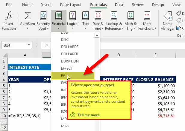
Now, this can be directly calculated using the FV function in Excel, where
- Rate = 10%
- NPER = 5 years
- PMT = Deposited amount each year ($1000.00)
- PV = present value (0)
- TYPE = 0 and 1 (0 means payment received at the end of the period, 1 payment received at the beginning of the period); in this scenario, it is 1
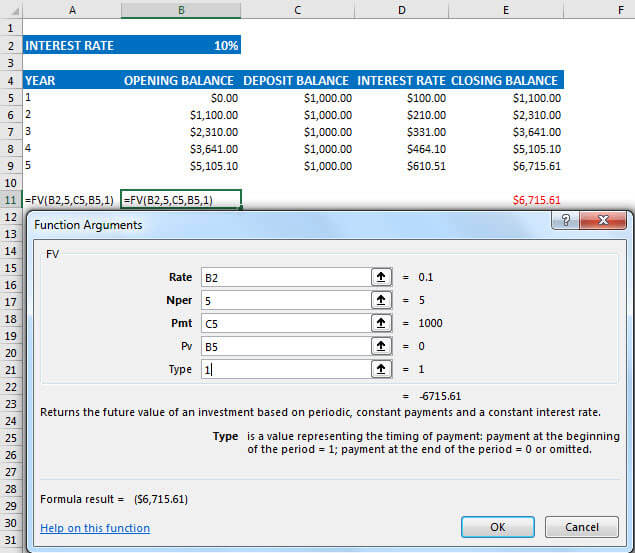
Here, the type is 1 because we receive the payment at the start of each period. The FV value calculated using the FV Function in Excel is within the red parenthesis that denotes the negative value. It is usually negative because, in the end, the bank is paying out the amount; thus, it signifies the outflow and inflow of the amount.
Example #2
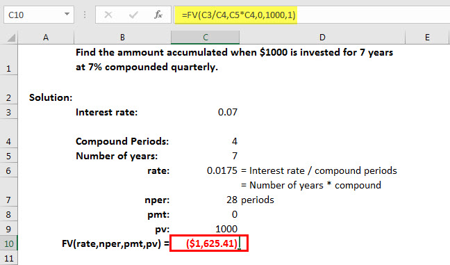
Calculate the accumulated amount when investing $1000 for 7 years at 7% compounded quarterly using Excel.
Interest rate: 0.07
Compound Periods: 4
Number of years: 7
Rate: 0.0175 = Interest rate/compound periods
nper: 28 = Number of years * compound periods
Pmt: 0
Pv: 1000
FV (rate, nper, Pmt, PV) = ($1,625.41)
You can download this FV function in the Excel template here – FV Function Excel Template.
Recommended Articles
This has been a guide to FV Function in Excel. Here we discuss the FV Formula in Excel and how to use FV in Excel, and practical examples and downloadable excel templates. You can also go through our other suggested articles –
