The Formula for Grade in Excel
The formula for grades in Excel involves using functions such as IF, Nested IF, AND, and OR to evaluate a student’s scores and calculate their grade. It benefits educators, teachers, and students who wish to monitor their academic progress and determine their grades for a subject.
To use the formula for the grade in Excel, a combination of logical functions (IF, Nested IF, AND, OR) and operators such as “>=, <=, >, <, =” must be employed. According to the grading system, these functions and operators help assign a proper grade.
How to use Formula for Calculating Grade in Excel?
Let us learn how to calculate letter grades and percentage-based grades in Excel using various functions with the help of different examples.
Example #1
Using the “IF” Function for a Single Condition
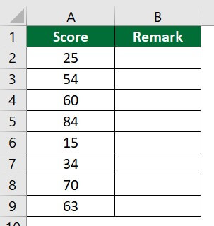
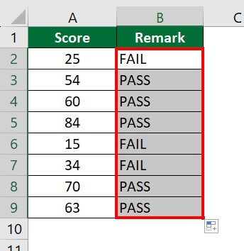
Consider the following data of scores of students. Here, we must assign remarks like pass or fail for the corresponding score. If the score is above 35, the remark should be “PASS”. If it is below 35, the function should display “FAIL”.
Solution:
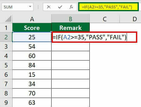
Step 1: Select “Cell B2” and enter the formula “=IF(A2>=35, “PASS”, “FAIL”)”.
Explanation of formula:
This formula will return “PASS” if the value of Cell A2 is greater than 35 and “FAIL” if the value is less than 35.
Step 2: Press “Enter“.
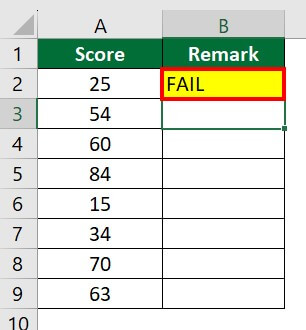
The function will display “FAIL” in Cell B2.
Step 3: Drag Cell B2 downward.
Let us calculate letter grades based on score values with the following examples.
Alternative to Excel Grade Formulas: Online Grade Calculators
While Excel formulas such as IF, Nested IF, and VLOOKUP are powerful tools for calculating grades, they require some familiarity with spreadsheet functions. For educators and teachers seeking a faster, simpler solution, online grading tools can be a great alternative.
One such tool is the ez grader calculator, a free online tool specifically designed for teachers to calculate student grades instantly, without writing a single formula. It works similarly to the traditional paper EZ Grader used in classrooms, but in a digital format.
When should you use an online grade calculator instead of Excel?
- When you need to grade a small quiz or test quickly
- When you don’t have Excel available on your device
- When you want to avoid complex nested formulas
- When you’re a teacher who prefers a dedicated grading tool over a general spreadsheet
For larger datasets or automated grade sheets, Excel formulas remain the best choice. However, for quick one-time calculations, an ez grader calculator saves significant time and effort.
Example #2
Using the “Nested IF” Function
The IF function in Excel can also be combined with AND/OR. In the earlier example, we used only the “IF” function for a single condition. For multiple conditions, we can use the “Nested IF” function.
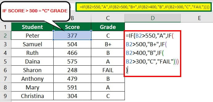
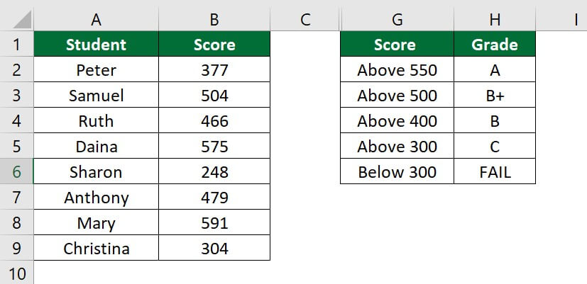
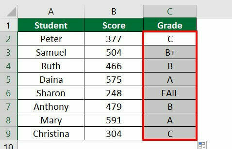
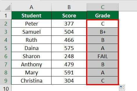
In the below example of a formula for a grade in Excel, we have data on students’ total marks, and we want to calculate the grades for the obtained marks. The following are the criteria for grades:
- If the Score is above 550, then the grade will be A
- If the Score is above 500, then the grade will be B+
- If the Score is above 400, then the grade will be B
- If the Score is above 300, then the grade will be C
- If the Score is below 300, the remark will be “FAIL”.
Follow the steps below to calculate students’ grades using the “Nested IF” function.
Solution:
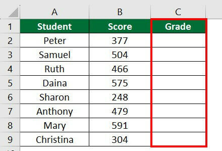
Step 1: Insert a new column beside the score column, as shown below.
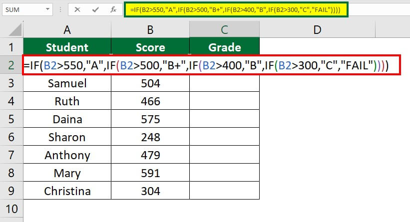
Step 2: Select “Cell C2” and enter the formula
“=IF(B2>550,”A”,IF(B2>500,”B+”,IF(B2>400,”B”,IF(B2>300,”C”,”FAIL”))))”.
Explanation of formula:
IF(B2>550, “A): If the score is more than 550, then the student will get an A grade.
IF(B2>500, “B+” ): If the score is more than 500, then the student will get a B+ grade.
IF(B2>400, “B” ): If the score is more than 400, then the student will get a B grade.
IF(B2>300, “C” ): If the score is more than 300, then the student will get a C grade.
“FAIL”: If none of the above conditions are met, the function will display “FAIL”.
Step 3: Press “Enter”.
The formula will display a “C” grade.
Step 4: Drag the bottom corner of Cell C2 to get grades for all the scores.
Example #3
Using the “IFS” Function
The “IFS” function in Excel also helps to calculate the letter grades. Let’s see how it works with the help of our previous example.
Solution:
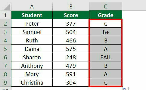
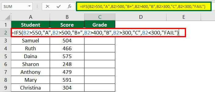
Step 1: Select “Cell C2” and enter the formula
“=IFS(B2>550,”A”,B2>500,”B+”,B2>400,”B”,B2>300,”C”,B2<300,”FAIL”)”.
Explanation of the formula:
The “IFS” function quickly checks multiple conditions and returns the corresponding value to the first TRUE condition. However, properly defining the source dataset is crucial for optimal data analysis. The formula states that if the value of Cell B2>550, then display “A”. If the value exceeds 500, display “B+”, and so on.
Step 2: Press “Enter”.
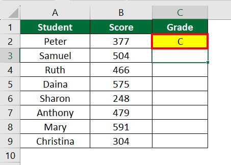
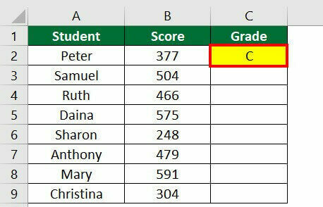
The formula will display “C”, as shown below.
Step 3: Drag the cell downward, as shown below.
Example #4
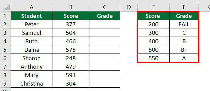
Using the “VLOOKUP” Function
If the above “Nested IF” and “IFS” function is difficult for you to understand, the VLOOKUP function in Excel is simple to understand and apply. Let’s calculate the letter grade with the “VLOOKUP” function.
Tips: Before using the VLOOKUP function, remember the following points
- Always create a lookup table as shown below because the VLOOKUP function will fetch results from the table_array.
- Change the score from “Above 550” to single numbers “550” (in Column E below), as VLOOKUP identifies a sequence of numbers as a table_array.
- Always sort the data in the table in ascending order to avoid errors.
Solution:
Step 1: Select “Cell C2” and enter the formula “=VLOOKUP(B2,$E$2:$F$6,2,TRUE)”.
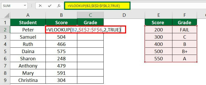
Explanation of the formula:
- B2 is the cell reference (lookup_value) or value that we want to look up.
- $E$2:$F$6 is the table range (table_array) from which the lookup value will be searched. The “$” dollar sign in the formula fixes the cells.
- 2 is the column number or column index in the lookup table from where the function will return the result.
- TRUE is to search for an approximate match.
The formula will search for the lookup value, i.e., “377” (value of Cell B2) in the lookup table range, “E2:F6“, and will return the approximate match from the corresponding column E, i.e., grade (Column F). If the function doesn’t find an exact match, it will return the value closest to or less than the lookup value. In our case, the exact match of 377 is not present in column E, so the function will look for the closest or lesser value than the lookup value(377), i.e., 300, and will return C, as shown below.
Step 2: Press “Enter”.
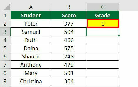
Step 3: Drag the cell to apply the same formula for all scores, as shown below.
Example #5
Using the “IF & AND” Function
In this method, we will determine grades based on individual student scores using Excel’s “IF & AND” function.
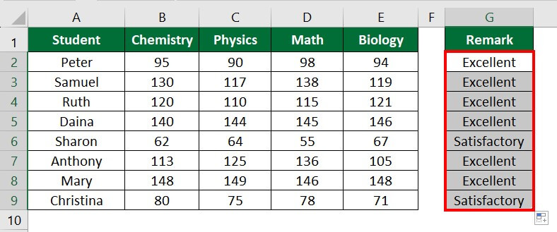
If a student scores 90 or above in all four subjects, their score will be considered “Excellent.” Otherwise, it’ll be considered “Satisfactory”. Let’s see how it works.
Solution:
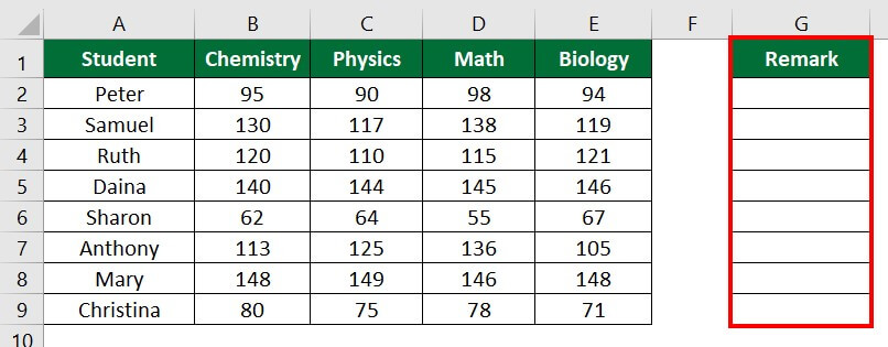
Step 1: Insert a new column, “Remark”, as shown below.
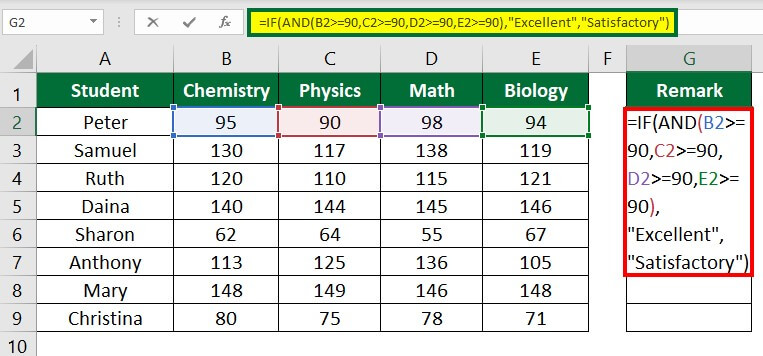
Step 2: Select “Cell G2” and enter the formula
“=IF(AND(B2>=90,C2>=90,D2>=90,E2>=90), “Excellent”, “Satisfactory”)“.
Explanation of formula:
The “IF” function returns a value when a condition is true. The function will also return another value if the condition is false for the selected cell. The condition is tested using the “AND” function, like if the student’s score is greater than or equal to 90. If all the conditions are correct, the function will result from a value of TRUE or else FALSE.
In our case, the formula states that if all values of Cell B2, C2, D2, and EC are more than or equals to 90, then the output will be “Excellent”, or else “Satisfactory”.
Step 3: Press “Enter”.
The output is displayed below.
Step 4: Drag the cell downwards, as shown below.

Example #6
Calculate Percentage-Based Grades in Excel Using “Nested IF” Functions
We will learn to calculate grades based on percentages using this method’s “Nested IF” function.
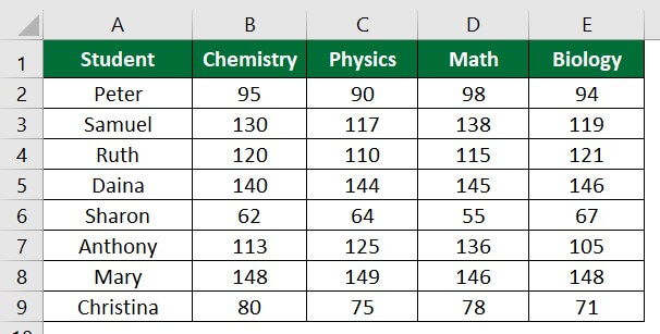
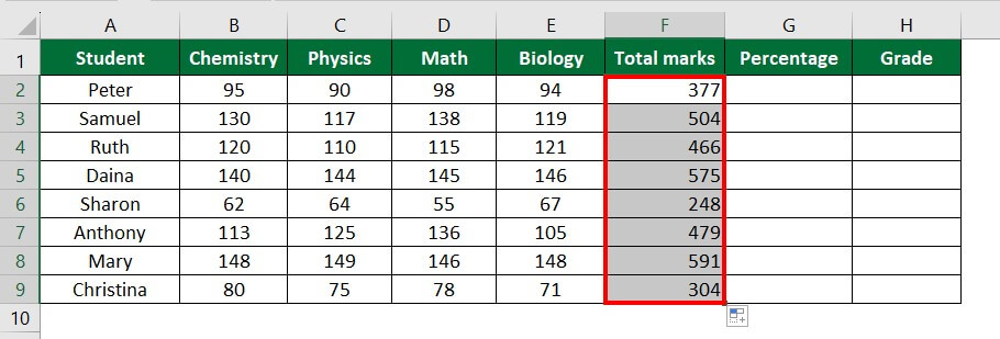
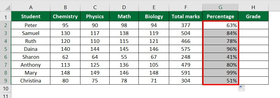
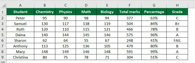
Consider the following data of students and their subject-wise marks. Here, we need to find out the percentage and grade for each student.

Solution
Step 1: Insert three columns, as shown below.
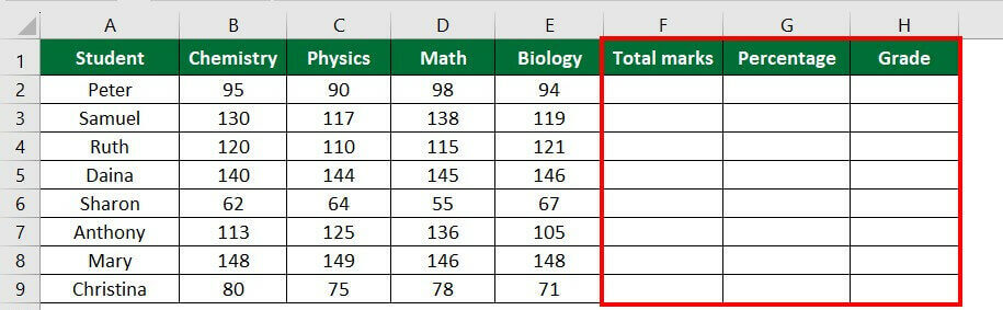
Calculate the total marks of students.
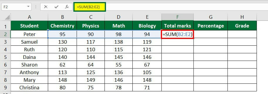
Step 2: Select “Cell F2“, enter the formula “=SUM(B2:E2),” and press “Enter”.
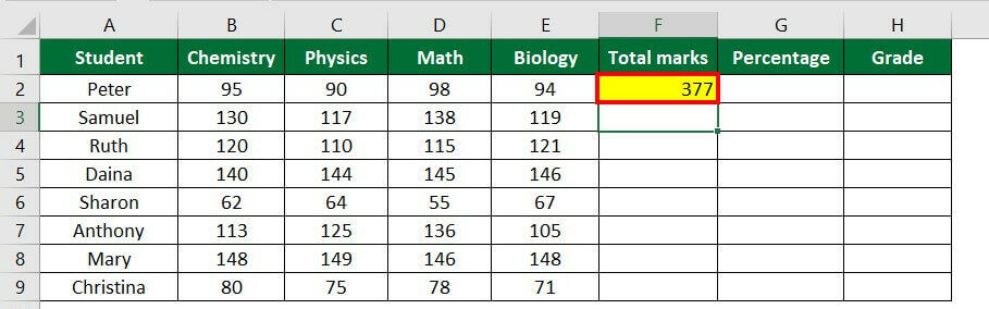
The SUM function “=SUM(B2:E2)” will return the total scores. Result 377 is displayed in Cell F2, as shown below.
Step 3: Drag the cell downwards, as shown below.
Calculate the percentage of students.
Step 4: Select “Cell G2” and enter the formula “=F2/600”.
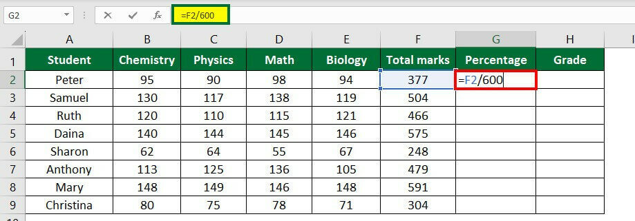
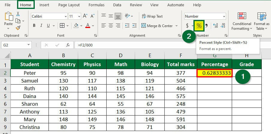
The formula “=F2/600” gives a decimal number like 0.68233333. To convert decimals to percentages, follow the below step.
Step 5: Select “Cell G2”, go to the “Home” tab and click on the “%” sign under the “Number” group, as shown below.
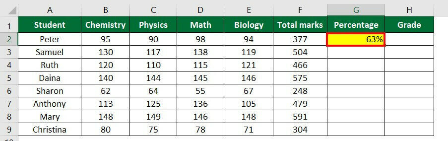
Step 6: Press “Enter”.
The decimal value gets converted into a percentage; see the below image.
Step 7: Drag the cell downwards, as shown below.
Calculate the grade for each student.
Step 8: Select “Cell H2” and enter the formula “=IF(G2>90%,”A”,IF(G2>80%,”B+”,IF(G2>=70%,”B”,IF(G2>=50%,”C”,”FAIL”))))”.
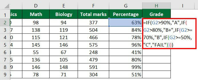
The “IF” function decides if the specified condition is met and then displays the defined output according to the condition.
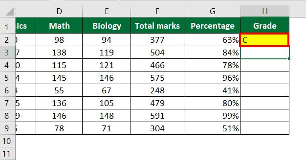
Step 9: Press “Enter”.
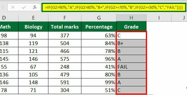
Step 10: Drag Cell G2 downwards to apply the formula for all cells.
Things to Remember
The below table offers helpful tips and examples for using formulas to calculate grades in Excel.
|
Tips |
Example |
| Enclose all text values with double quotes. | “Olivia”, “English” |
| Numerical values need not be enclosed with double quotes. | 50, 2.5 |
| Use IF & AND conditions to check if all conditions are true.
For instance, use this formula to check if a student scored above 80 marks in all subjects. |
IF(AND(A1>=80, B1>=80, C1>=80, D1>=80), “Excellent”, “Satisfactory”) |
| Use IF & OR conditions to check if any one condition is true.
For instance, to check if a student scored above 80 marks in any one subject, use this formula: |
IF(OR(A1>=80, B1>=80, C1>=80, D1>=80), “Yes”, “No”) |
| Close formula with brackets equal to the number of IF statements.
If the formula has two nested IFs, it should be closed with two closing brackets like this: |
=IF(A1>=85, “A”, IF(A1>=75, “B”, “C”)) |
| When using the “VLOOKUP” function, the marks/score table column should be in ascending order, or the function can give an error or wrong result. | – |
| In the last argument of the VLOOKUP function, use “TRUE” or 1 for an approximate match. | VLOOKUP(B2,C2:E10,2,TRUE) |
Recommended Articles
This has been a guide to Formula for Grade in Excel. Here we discussed How to use Formula for Grade Calculation in Excel, practical examples, and a downloadable Excel template. You can also go through our other suggested articles –
