Updated May 8, 2023
Rounding in Excel
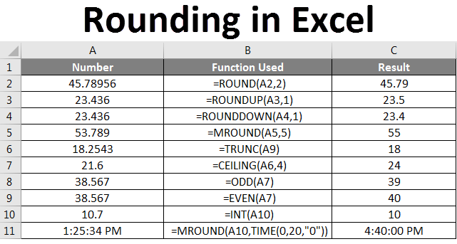
Rounding in Excel alters the actual value in a cell. In simple words, rounding means eliminating unwanted numbers and keeping the nearest numbers. A simple example will make you understand better. The rounding value of 99.50 roundings is 100. We have different kinds of rounding functions available to make rounding as per requirements.
How to Round Numbers in Excel?
Let’s understand how to Round Numbers in Excel using various functions, with examples explained below.
ROUND Function
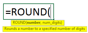
Round is the first function that strikes us when considering rounding in Excel. The round function makes rounding of numbers as per the number of digits we want to make rounding.
Syntax of ROUND is =ROUND(number, number_digit). Find the below screenshot for reference.
Suppose there is a number 45.78956 in cell A2, and we wish to have only 2 digits after the decimal point. Apply the ROUND function with number_digits as 2.
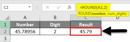
Observe the screenshot .78956 converted to 79 as we mentioned 2 in the number of digits after the decimal point; hence it makes rounding to nearer number .79
ROUNDUP Function
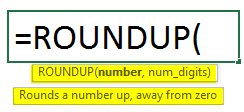
Roundup name itself suggests that this function rounds the number upwards only.
The syntax for ROUNDUP Function is =ROUNDUP(number, number_digits). Find the below screenshot for reference.
The number of digits it will take upward depends on the number of digits we give in the “number_digit” during the input roundup formula.
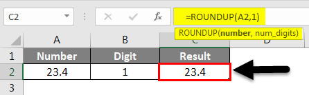
In the above screenshot, there is only one value after the decimal point, and we also give 1 in the formula; hence, the results are not changed. Suppose we increase the number of digits after the decimal point as below.
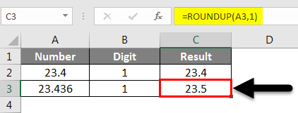
23.436 rounded as 23.5 as after decimal there should be only one digit; hence it makes rounding to its upper value and make as 23.5
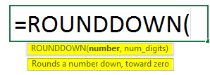
ROUNDDOWN Function
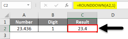
The syntax for ROUNDUP Function is =ROUNDUP(number, number_digits). It is quite the opposite of ROUNDUP, as it rounds to a lower value and displays the number of digits the user mentions after the decimal point. Find the below screenshot for reference.
Consider the same example used for ROUNDUP; there, we got the result as 23.5, and here we got the result as 23.4 as it is rounded to the lower value.
MROUND Function
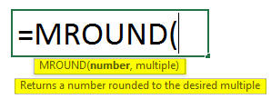
MROUND function performs rounding, which may go up or down depending on the given multiple in the formula.
The syntax of MROUND is =MROUND(number, multiple). Find the below screenshot for reference.
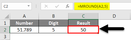
In the below example, we use a multiple of 5; hence the results should be multiple of 5. 50 is the nearest multiple value of 5 for 51.789
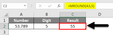
In the example below, 55 is the nearest multiple value of 5 for 53.789.
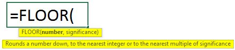
FLOOR Function
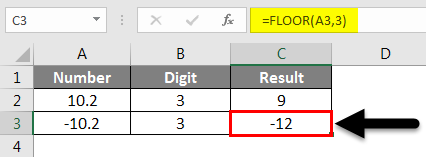
The floor is another function that helps to round off numbers down. The syntax of the FLOOR Function is =FLOOR(number, significance). Find the below screenshot for reference.
We want to do rounding; significance is the number we want to do the multiple. In the below example, we want the multiple of 3; hence we have given 3 in the place of significance. 9 is the nearest multiple of 3 for the value 10.20.

We can perform this for negative values too; as told earlier, it helps to down the number; hence it gives the result as -12 because if we reduce -10.20 further, -12 is the nearest multiple of 3; therefore, it is -12.
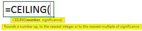
CEILING Function
CEILING is another function of rounding up the numbers. The syntax for the CEILING Function is =CEILING(number, significance). Find the below screenshot for reference.
It is similar to the FLOOR Function, but the difference is that it is used for Round Down, which is used for Roundup.
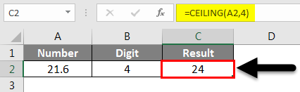
In the below example, we have given the significance as 4, which means we need a rounding value greater than 21.60 and should be a multiple of 4. 24 is greater than 21.6, and it is a multiple of 4.
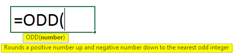
ODD Function
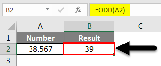
The ODD function is one of the rounding functions that help to find the nearest odd number of the given number.
The syntax for ODD is =ODD(number).
In the below example, we applied the ODD function for number 38.567. 39 is the nearest Odd number available hence it gave the result as 39.
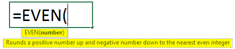
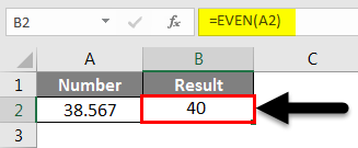
EVEN Function
Even function works quite similarly to the ODD function, but the only difference is that it gives the nearest EVEN numbers after rounding.
Syntax of EVEN is =EVEN(number).
Find the below example for reference. The nearest number for 38.567 is 40.
TRUNC Function
TRUNC is another function available for rounding numbers. The syntax for TRUNCATE Function is =TRUNC(number, [number_digits])
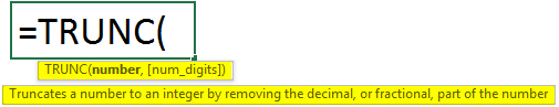
As through the number of digits, it will eliminate numbers after the decimal point. It will round to the nearest integer if we do not provide any number.
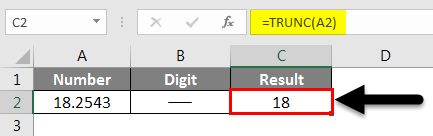
Observe the above screenshot; TRUNC is applied without several digits. 18 is the nearest integer of 18.2543.
Now we will see how it will work if we give the number of digits as 2 for the same example.
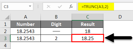
It keeps only two values after the decimal point and truncates the other digits. If we give the number a positive number, it will truncate from the right side of the decimal point. If we give negative values and negative numbers, it will truncate from the left side of the decimal point.
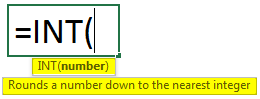
INT Function
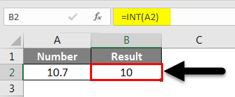
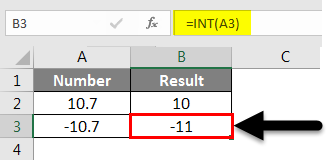
INT is another function that rounds the value down to the nearest integer. Syntax of INT is =INT(number)
If we use a positive value or negative value, it will always be rounding down the value. Even if we use 10.7; still, it downs the value to the nearest integer, 10.
Perform the same for the negative value now. Observe below it further reduces the value of 10.70 to -11.
ROUNDING for TIME
Rounding can apply to time also. We will see a few examples of rounding the time. The syntax for rounding the time is =CEILING(time, “1:00”). Find the below screenshot for reference.
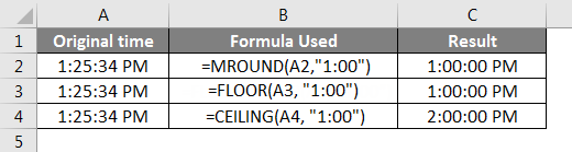
Observe the above formula; similarly, I applied for FLOOR and CEILING.
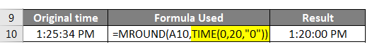
We have to follow a different format if we want the rounding nearer to 20 minutes like that. Please find the below screenshot for rounding to the nearest 20 minutes.
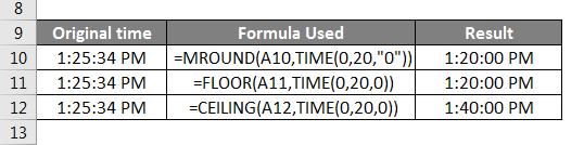
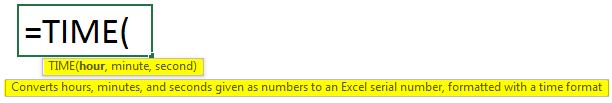
Observe the formula; the moment we give the time, it will ask for hours, minutes, and seconds; hence we can give the nearest time details for rounding. Below is the syntax for that.
I hope you understand how to apply rounding formulas differently per the situation.
Things to Remember While Using Rounding in Excel
- ROUNDUP and ROUNDDOWN can be applied for negative numbers too.
- If we use positive numbers and negative significance, the results will be #NUM, like an error message for CEILING and FLOOR Functions.
- Rounding can also be applied to time while working with the time input formula as per minutes and hours.
Recommended Articles
This has been a guide to Rounding in Excel. Here we discussed How to Round Numbers, Time using functions like ROUND, ROUNDDOWN, CEILING, FLOOR, INT, TRUNC, etc., in Excel, along with practical examples and a downloadable Excel template. You can also go through our other suggested articles –
