Updated May 9, 2023
What is MROUND in Excel?
MROUND is an Excel function categorized under math & trigonometric function in Excel. Commonly this function is used with numeric values. The function operates in such a way as to round the supplied number up or down to a mentioned multiple within the formula. This function can be used to round a number according to a multiple. According to the different situations, this will round the number towards 0 or away from 0.
Syntax:
Arguments of MROUND Function:
- Number: The numerical value you want to convert or round.
- Multiple: The multiple to which you round the specified number.
If you look at the process or how it operates among the provided data, the MROUND function will round your number supplied into a perfect multiple up or down to the given multiple. Per the condition, the multiple can select towards 0 or away from 0. You might need clarification about how this can be selected, the criteria to select a multiple greater than the number to be rounded, and what it will be to select a number less than the given number. For this, you can refer to the two conditions explained below. The given number will fall in any of the below conditions.
- Divide the number you want to round with the multiple. If the remainder is greater than or equal to half of the multiple, then round the number up.
- Divide the number you want to round with the multiple if the remainder is less than or equal to half of the multiple, round the number down.
Suppose the formula applied is MROUND= (7,4). This rounds the number 7 into the nearest multiple of 4. The result will be 8. For more clarification, you can go through the detailed examples.
How to Apply MROUND Function in Excel?
Let’s understand how to apply the MROUND in Excel with some examples.
Example #1 – Rounding Up Multiple of a Number
Before getting into complicated calculations, let’s learn the logic of the MROUND function. For example, you have given the number 15 and want to round it into the multiple of 6. So the formula applied will be:
MROUND= (15,6)
You may need clarification about whether the number round into 18 or 12. 18 is the nearest multiple of 6 away from 0, and 12 is also a multiple toward 0. Both are two nearest multiple up (away from 0) and down (towards 0) to the number you want to round. So which number could you select as a result? In such a situation, you can go through the two conditions below and select the appropriate condition for the data given.
Divide 15, the number you want to round, with the multiple 6. It depends on the value of the remainder to select the condition.
- If the remainder is greater than or equal to half of the multiple, then round the number away from zero.
- If the remainder is less than the multiple, then round the number, which is toward zero.
Here the remainder is 3. Check whether the reminder is greater than or equal to half of the multiple. Multiple is 6, and half of the multiple is 3; in this situation, you can go ahead with the first condition, round the number up or away from zero.
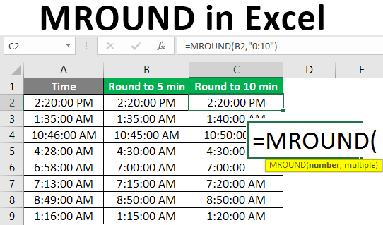
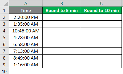
Example 2: Rounding Times
You can apply the MROUND to the nearest 5 and 10 minutes. The time is provided, and let’s apply the formula to it.
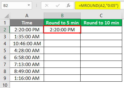
- The time is given in (hh: mm: ss AM/PM) format, so the minute is mentioned as “0:05” in the formula. The formula is ‘=MROUND(A2, “0:05”)’. If the result shows, some other values change the format to time as you are given the time format.
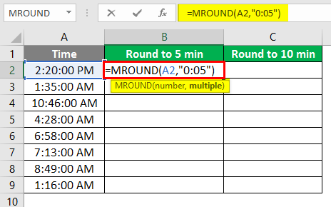
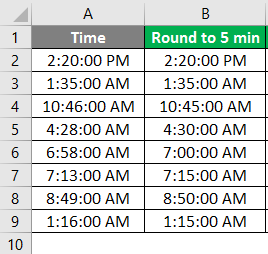
- After applying the formula, the answer is shown below.
- Drag the same formula in cell B2 to B9.
- The results are rounded accordingly, and the result is calculated depending on the same rules of the reminder value.
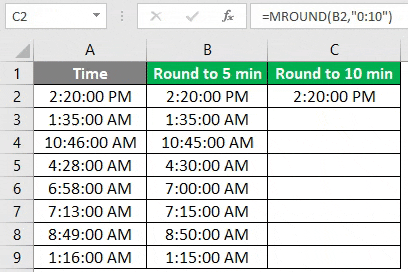
- In the same way, 10 minutes is rounded, and the formula is ‘=MROUND(B2, “0:10”)’.
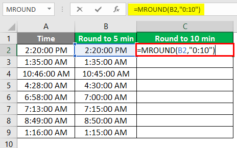
- After applying the formula, the answer is shown below.
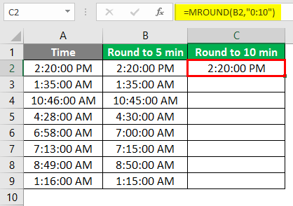
- We will be applying the same formula to entire cells, and the final result is as shown:
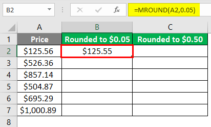
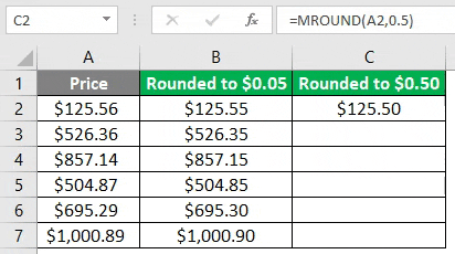
Example #3 – MROUND Function on Price
Through this example, you can learn how the MROUND function can be used to round the fraction of the price or amount while making billing towards a large amount. This is used to provide discounts on the fraction of the amount of rounding the amount into a perfect figure.
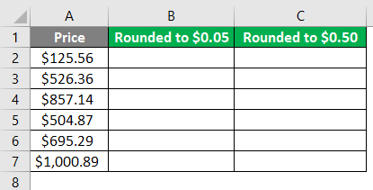
- In a big deal of amounts, to avoid the small sum of prices, you can use this MROUND function. This method is effective for applying according to the discounts you provide or a fraction of the amount you want to neglect. The formula applied is ‘=MROUND(A2,0.05).’
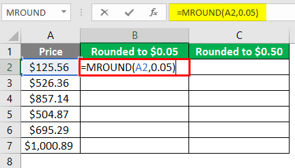
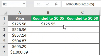
- After applying the formula, the answer is shown below.
- Drag the same formula in cell B2 to B7.
- Apply the below formula in cell C2.
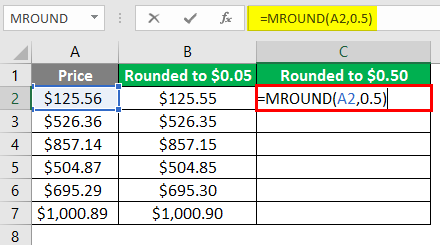
- After applying the formula, the answer is shown below.
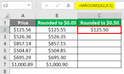
- Drag the same formula in cells C2 to C7.
Things to Remember About MROUND in Excel
- MROUND function works only with numbers; both arguments should be numbers.
- #NAME?” will be the error produced if any parameters are not numeric.
- If signs like positive or negative are used along with any of the parameters, it will show an error “#NUM!”.
Recommended Articles
This is a guide to MROUND in Excel. Here we discuss how to apply MROUND in Excel, practical examples, and a downloadable Excel template. You can also go through our other suggested articles –
