Updated May 8, 2023
Running Total in Excel
Running Total is a form of Cumulative Sum process in Excel that matches the total sum obtained using the traditional SUM function or addition process with the previous cell value sum with the current cell value. For example, we have 5 numbers whose sum is 100. To confirm whether all the values are considered in the addition process, we will sum the 2nd Value with the 1st value. Then, keep summing the previously obtained sum and the value of the previous cell. If Cumulative Sum and traditional sum summation come equally, then there is no cell left or no discrepancy in the selected data.
Methods to Find Running Total in Excel
In this article, I will cover how to find running totals in Excel. There are several ways we can find the running total in Excel. Follow this article, explore each of them, and add skills to your CV.
Running Total by SUM Function in Excel – Method #1
We can find the running total by using the SUM function. I have sales data day-wise for one month, i.e., Jan 2018, and a few days’ data from Feb.
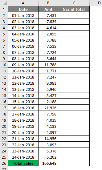
I have a total at the end. This gives me an overall picture of the month. But if I want to know which day made the difference, I cannot tell with the overall sum. So I need a running total or cumulative total to tell the exact impact date.
By applying the SUM function, we can find out the running total.
- Open the SUM function in the C2 cell and select the B2 cell.
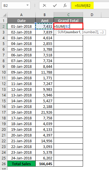
- Now press the colon ( : ) symbol and select cell B2.
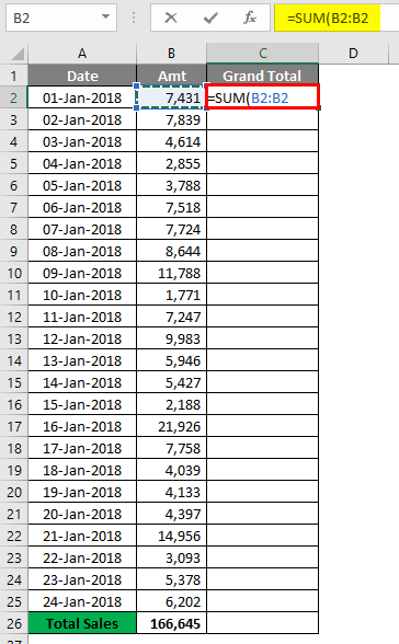
- Select the first B2 value and press the F4 key to make it an absolute reference.
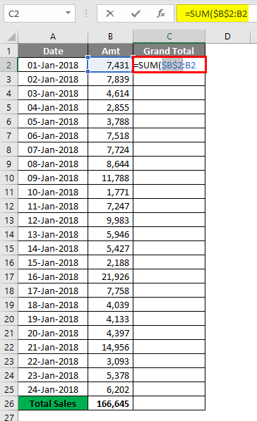
- The result will be as given below.
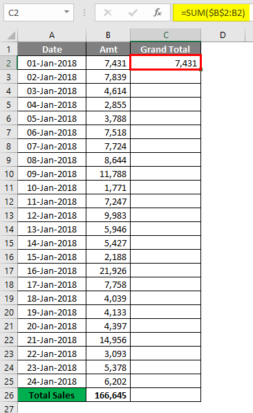
So now the first B2 cell with the dollar symbol becomes an absolute reference; when we copied down the formula, the first B2 cell remains constant, and the second B2 cell keeps changing with B2, B4, B5, and so on.
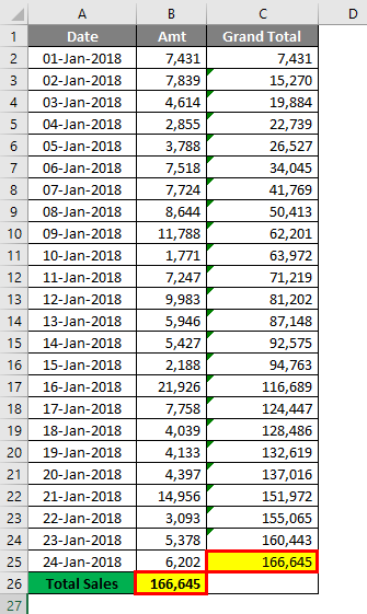
- Drag the formula to the remaining cells to get the running total.
- Now the total and the last running total are both the same.
Like this, we can get the running total by using the SUM function. Let’s apply a cumulative graph to the table to find the exact impact.
Select the data under the Insert tab Insert Column chart.
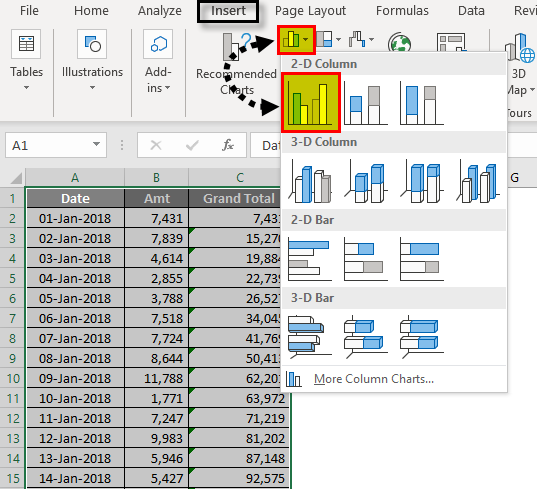
- As soon as you insert the chart, it will look like this.
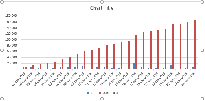
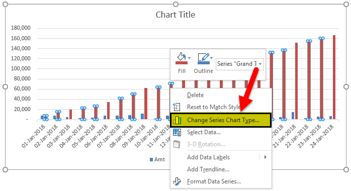
- Now select the total grand bar and select Change Series Chart Type.
- Change the chart type to LINE chart and then click Ok.
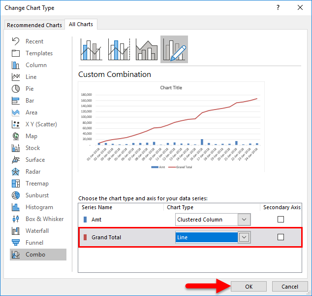
- A line graph represents the total, and a bar graph presents daily sales.
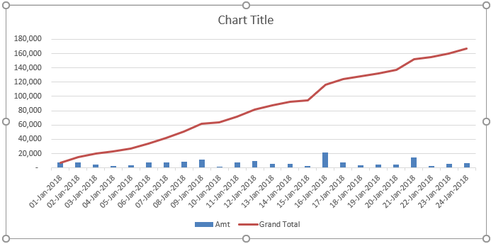
On 16th Jan 2018, we can see the impact. On that date, revenue increased by 21926.
Running Total by Pivot Table in Excel – Method #2
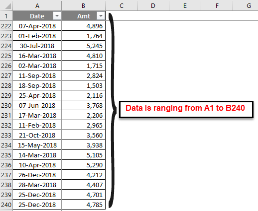
We can find the running total by using Pivot Table as well. I use slightly different data from the daily sales tracker for this example. Data ranges from Jan to Dec.
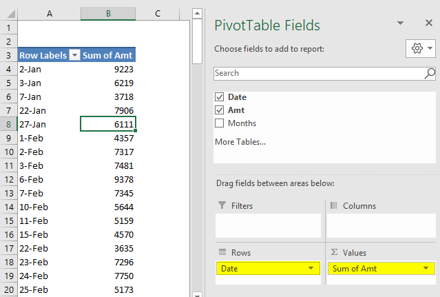
Let’s apply the pivot table to this data. First, apply the pivot table date-wise, as shown in the image below.
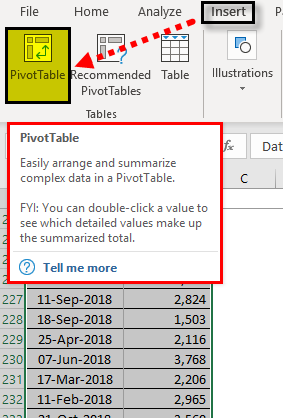
- Go to Insert Tab and then click on the Pivot Table.
- Drag Date Field to Rows section and Amt to Value section.
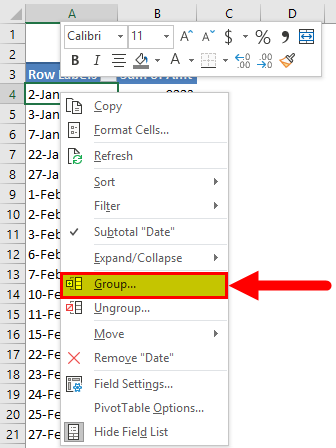
- Now group all the dates into months. Right-click on the date and select GROUP.
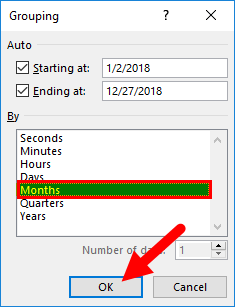
- Under Grouping, select Months as the option. The Excel pivot table itself automatically selects starting date and the ending date. Click on OK to complete the process.
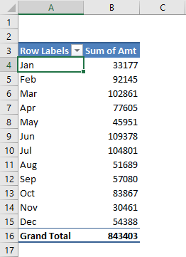
- Now we have grouped all the dates into respective months and have a monthly total instead of a day-wise total.
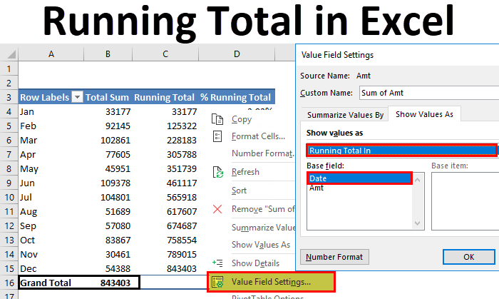
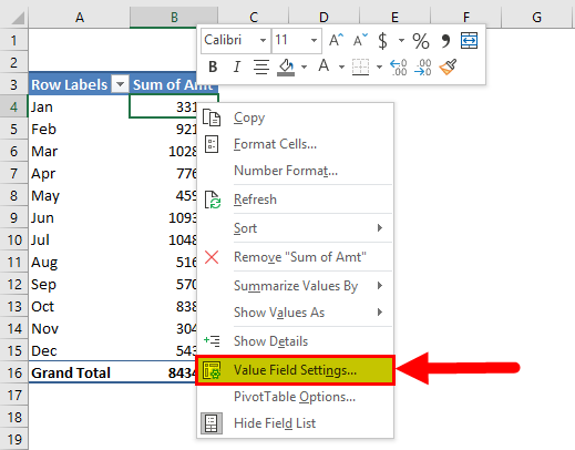
- Now right click on the column total and select Value Field Settings.
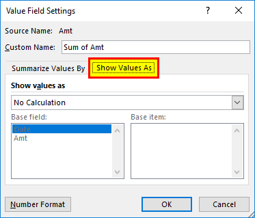
- Now under Value Filed Settings, select Show Values As.
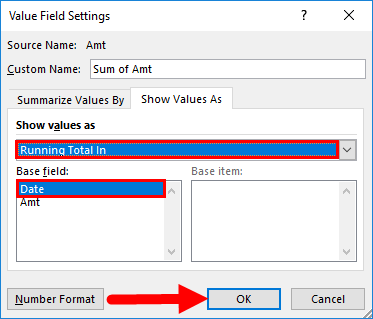
- From the drop-down list, select Running Total and select Date as the Base Field, and then click on Ok to complete the process.
- We have a running total now.
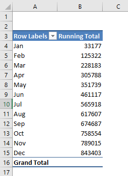
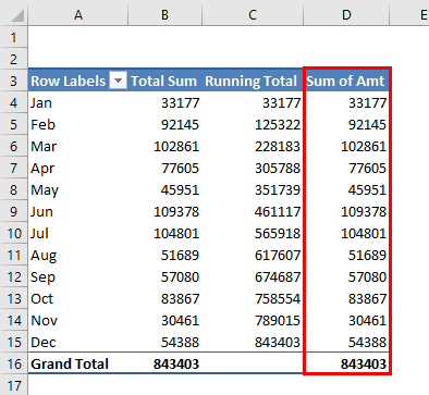
- The problem is we do not have a total sale column here. So, to show both the running and month-wise total, add the sales amount again to the VALUES.
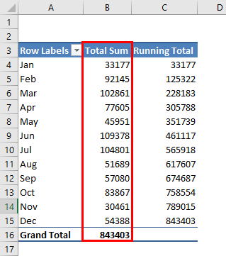
Now we have both total sums and the Running total in place.
Add Percentage Running Total in Excel.
Excel does not stop there only. We can add a total running percentage as well. To add the % running total, add one more time amt column to Values.
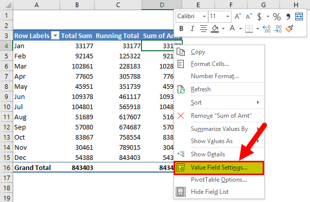
Now right click on the newly inserted column and select Value Field Settings.
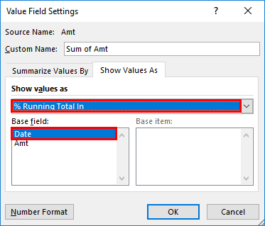
Now under this Value Field Settings, go to Show Values As. Under this, select Running Total %.
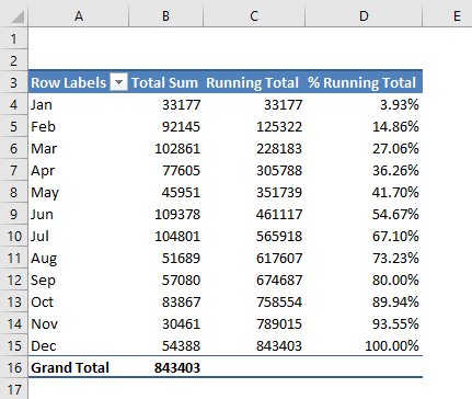
Finally, name this as % Running Total.
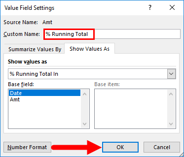
Click on Ok to complete the process. Now we have Running Total and % Running Total along with the monthly sales amount.
Things to Remember
- Running total is dynamic in the pivot table; if there is any change in the main data running total changes accordingly.
- To show the running and monthly total together, we need the sales amount column to the VALUES twice. Therefore, one will be for monthly sales and another for Running Total.
- By adding a graph, we see the impactful changes visually.
Recommended Articles
This has been a guide to Running Total in Excel. Here we discuss the methods to find the running total in Excel, examples, and downloadable Excel templates. You can also go through our other suggested articles to learn more –
