Updated April 29, 2023
FLOOR Function in Excel (Table of Contents)
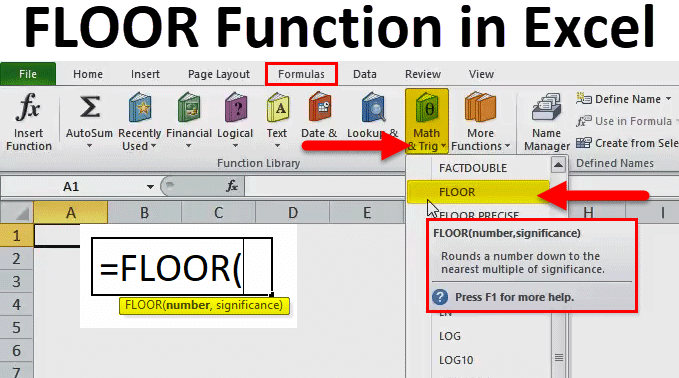
FLOOR in Excel
The floor function is used for rounding down the decimal and integer numbers. Still, this function converts the selected numbers to the nearest specified numbers to any down value. For example, if we have a number 10 that we need to round, multiple values should be down less than 2 to see the change as per syntax significance. If we select 3 instead of significance multiple, we will see a round down to the nearest 3 as 9.
FLOOR Formula in Excel:
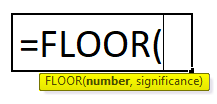
Below is the FLOOR Formula in Excel.
Explanation of FLOOR Function in Excel:
The FLOOR formula in Excel has two arguments.
- Number: It is a number you want to, or we want to round.
- Significance: It is multiple to which you wish to round the number.
How to Use the FLOOR Function in Excel?
The FLOOR function in Excel is very simple and easy to use. Let us understand the working of the FLOOR function in Excel by some FLOOR Formula examples.
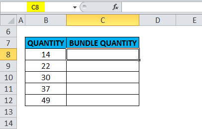
Example #1
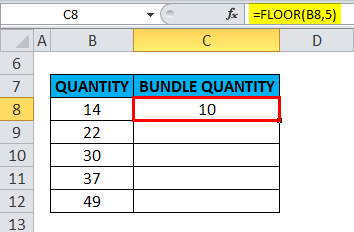
In this FLOOR function in Excel example, I have to sort out only complete bundles, i.e. bundles with only 5 quantities of a product. The quantities are as mentioned in column B; Now, I want to bundle them in multiples of 5 using the floor function in column C. Need to Follow the below-mentioned steps in Excel:
Select the output cell where we need to find the floor value, i.e. C8 in this example.
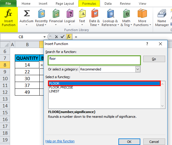
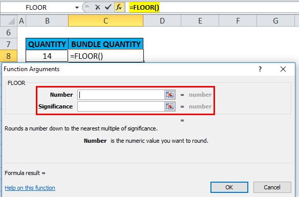
Click the insert function button (fx) under the formula toolbar. A dialog box will appear. Type the keyword “floor” in the search for a function box; the FLOOR function will appear in the Select a function box. Double-click on the FLOOR function.
A dialog box appears where arguments (Number & significance) for floor function need to be filled or entered.
Here, number one is 14; Whereas the significance value is 5, the Significance value is common to other cells.
Following FLOOR formula is applied in the C8 cell, i.e. =FLOOR(B8,5).
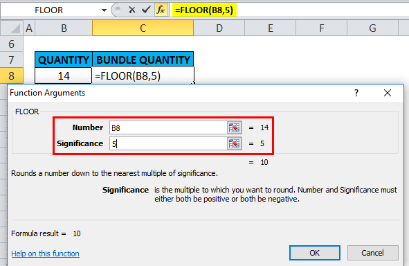
Output or Result: The value 14 is rounded to 10.
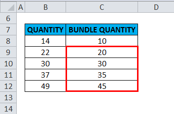
Similarly, it is applied to other cells in that column to get the desired output.
Example #2
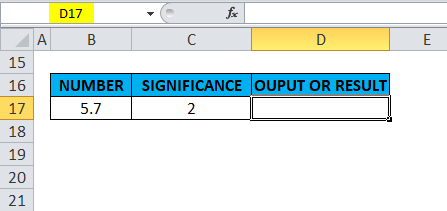
In the second example of the FLOOR function in Excel, the number argument is a decimal value in cell B17 & the significance value is 2 in cell C17. I need to find out the nearest multiple of 2 for the Decimal value of 5.7
Need to Follow the below-mentioned steps in Excel:
Select the output cell where we need to find the floor value, i.e. D17 in this example.
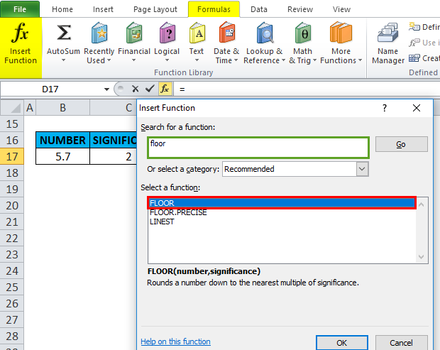
Click the insert function button (fx) under the formula toolbar. A dialog box will appear, type the keyword “floor” in the search for a function box, FLOOR function will appear in the select function box. Double-click on the FLOOR function.
A dialog box appears where arguments (Number & significance) for floor function need to be filled.

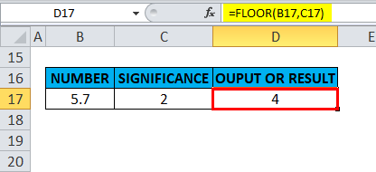
Here number argument is 5.7, Whereas the significance value is 2. Following floor, formula is applied in the D17 cell, i.e. =FLOOR(B17,C17)
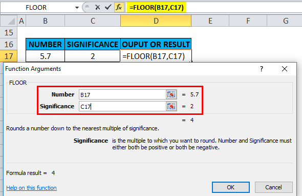
Output or Result: It Rounds 5.7 down to the nearest multiple of 2 and returns the value 4.
Example #3
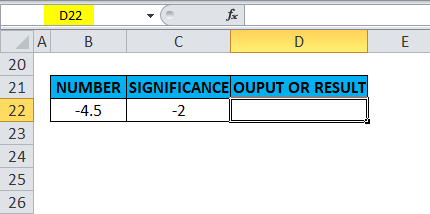
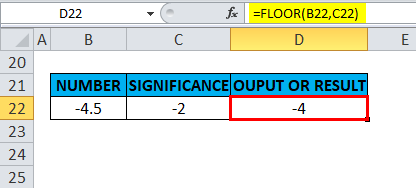
In the third example of the FLOOR function in Excel, the number argument is a negative value (-4.5) in cell B22 & the significance value is also negative (-2) in cell C22. I must find the nearest multiple of -2 for the number value -4.5.
Select the output cell where we need to find the floor value, i.e. D22 in this example.
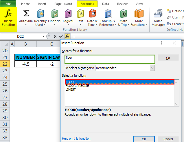
Click the insert function button (fx) under the formula toolbar; a dialog box will appear, type the keyword “floor” in the search for a function box, FLOOR function will appear in selecting a function box. Double-click on the FLOOR function.
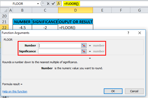
A dialog box appears where arguments (Number & significance) for floor function need to be filled.
Here, number one is -4.5, Whereas the significance value is -2, Both of which are negative. FLOOR formula is applied in a D22 cell, i.e. =FLOOR(B22,C22).
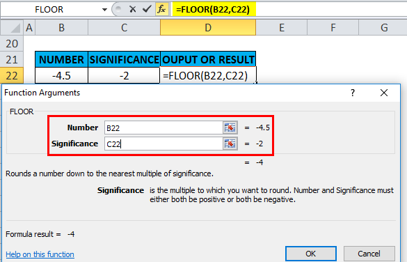
Output or Result: It Rounds -4.5 down to the nearest multiple of -2 and returns the value -4.
Example #4
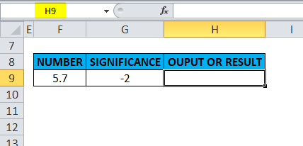
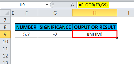
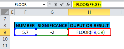
FLOOR function in Excel returns an #NUM! Error value if the number value is positive and the significance value is negative. In the below-mentioned example, the number argument is a positive value (5.7) in cell F9 & the significance value is a negative value (-2) in cell G9. I need to find the nearest multiple of -2 for the value 5.7.
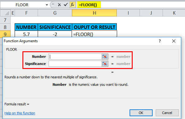
Select the output cell where we need to find the floor value, i.e. H9 in this example.
Click the insert function button (fx) under the formula toolbar; a dialog box will appear, type the keyword “floor” in the search for a function box, FLOOR function will appear in selecting a function box. Double-click on the floor function.

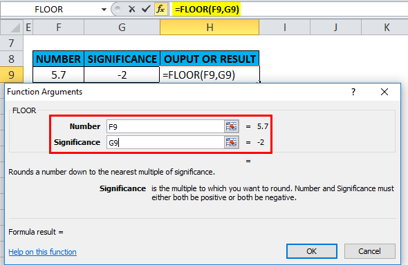
A dialog box appears where arguments (Number & significance) for floor function need to be filled.
Here number argument is 5.7, Whereas the significance value is -2
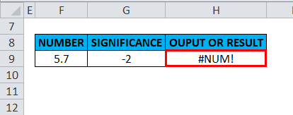
Following FLOOR function is applied in an H9 cell, i.e. =FLOOR(F9,G9).
Output or Result: FLOOR function returns an #NUM! Error value if the number is positive and significance is negative.
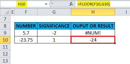
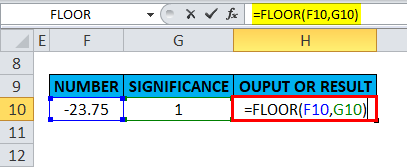
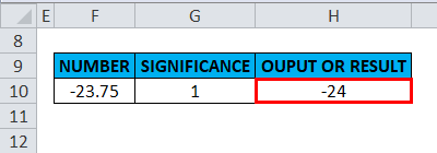
Whereas in the case if the number is negative and significance is a positive value. It can handle a negative number and positive significance in current versions of Excel 2016 & 2010 or later. #NUM! Error value will not occur. In the below-mentioned example, a negative number argument (-23.75) in cell F10 and a positive significance argument (1) in cell G10.
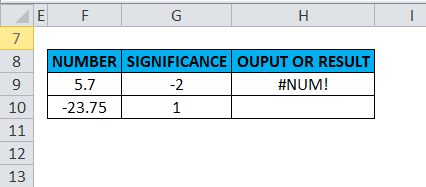
FLOOR Function in Excel reverses the negative number away from zero, i.e. it returns an output value as -24 (More negative value) in cell H10.
Things to Remember
The FLOOR Function in Excel performs rounding based on the below-mentioned or following rules:
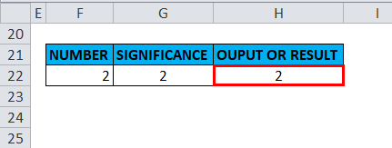
- No rounding occurs if the number argument is equal to an exact multiple of significance.
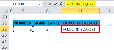
The Output will be :
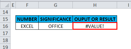
- If either argument ((number, significance) is non-numeric (Text value or string), the FLOOR function returns an #VALUE! Error.
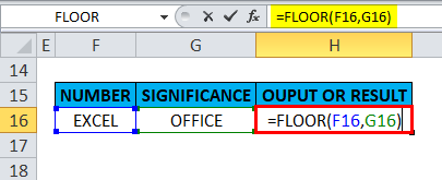
The Output will be :
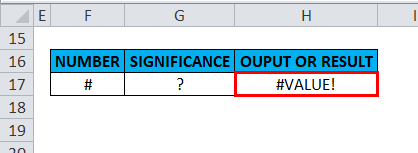
- If “number” or “significance” argument has different signs (e.g. #, %,?), the FLOOR function returns an #VALUE! Error.
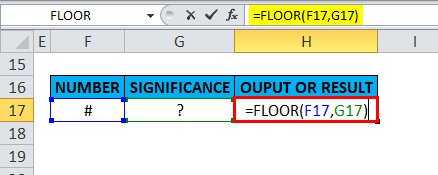
The Output will be :
- The significance & number argument must have the same arithmetic sign (positive or negative); otherwise, they have different arithmetic signs.
The Floor function returns or results in an #NUM error value.
- Exceptional case or scenario, In current versions of Excel 2016 or (2010 and later), a negative number argument (-23.75) in cell F10 and a positive significance argument (1) in cell G10 Floor function reverses the negative number away from zero, i.e. -24 in cell H10, if you try this it in Excel 2007 & earlier versions, it returns a value error (#NUM! error value)
The Output will be :
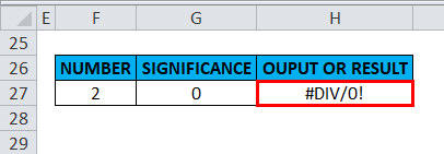
- If the number argument is a positive value and the significance argument is “0” or ZERO, it returns #DIV/0! Error.
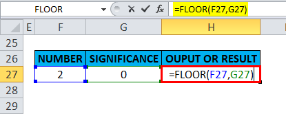
The Output will be :
Recommended Articles
This has been a guide to FLOOR in Excel. Here we discuss the FLOOR Formula in Excel and How to use the FLOOR Function in Excel, along with practical examples and a downloadable Excel template. You can also go through our other suggested articles –
