Updated June 7, 2023
Excel Negative Numbers (Table of Contents)
Introduction to Negative Numbers in Excel
Negative numbers are the ones that are lower than zero, and by default, they have a minus symbol as a prefix in Excel. These numbers are with your sales, margin, scores, and financial data occasionally, and you have to deal with those with care. Though it is quite easy and simple in Excel to deal with negative numbers, it may sometimes create confusion for the user due to the different visibility of the same under Excel. Especially a new user might have confused while working on those. But remember a simple rule: any number with a minus sign as a prefix is a negative number. There are various ways of representing/highlighting negative numbers in Excel.
Examples of Negative Numbers in Excel
Let’s understand how to use Negative Numbers in Excel with some Examples.
Example #1 – Negative Numbers with Conditional Formatting
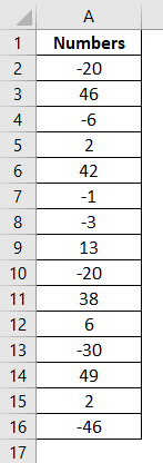
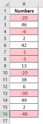
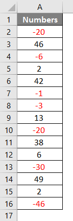
In representing negative numbers, we check whether the number in cells is less than zero. If the number is less than zero, it will be colored with a specific color. Suppose we have data, as shown below, consisting of positive and negative numbers.
To highlight the negative numbers, follow the steps below:
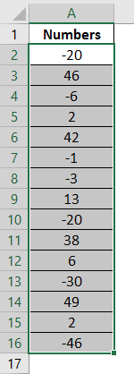
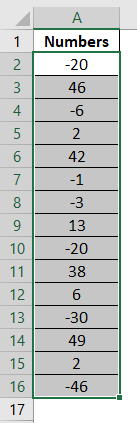
Step 1: Select all the cells containing your data. See the screenshot below for your reference:
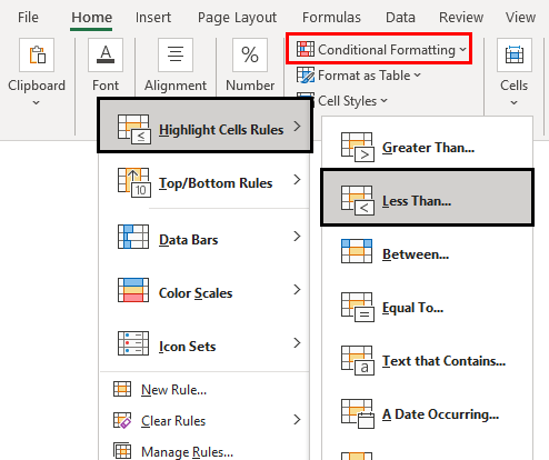
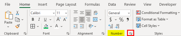
Step 2: Click the Home tab button on the Excel ribbon; you can see a Conditional Formatting dropdown under the Styles group.
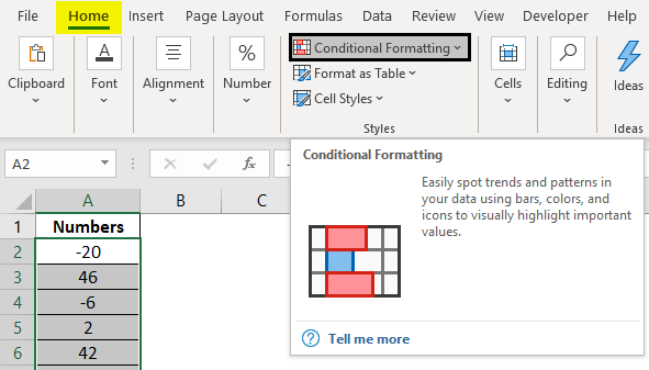
Step 3: Now, click on the Conditional Formatting dropdown, and you can see a list of options below. Navigate toward the Highlight Cell Rules, and there you can see the Less Than… rule. Click on it.
Step 4: A new dialog box, Less Than, opens up. In that box, Put the value as zero (0) within the box under Format cells that are Less Than and select appropriate cells and text color through the dropdown menu on the right.
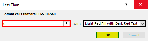
Click the OK button, and you can see the result below. Where all the negative numbers are colored Red and cells are colored light red.
Example #2 – Negative numbers with Built-in Number Formatting
Now we will see how to represent the negative numbers with the built-in number formatting in Excel.
Step 1: Select all the data from your cells as shown below:
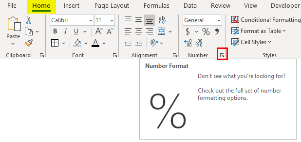
Step 2: Navigate to the Home tab under the Excel ribbon and click on the small arrow type icon, which is there to enlarge the number formatting under the Number group. See the screenshot below:
A new window will pop up named Format Cells. Here you can format the cells and customize the cell’s formatting as per your requirements.
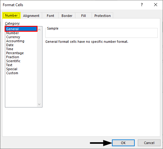
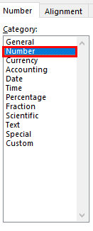
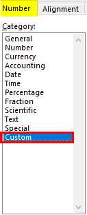
Step 3: By default, the Number tab gets highlighted inside the Format Cells window out of all six tabs. You need to click on it to select it if it is not. Under the Number tab, select Category: as Number.
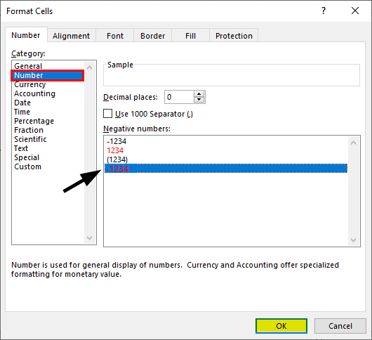
Step 4: Once you click on the Number option, on the right-hand side, under the Format Cells window, you can see a sample of the formatting. Reduce the Decimal Places: to zero (0) from 2 and Select the last numbering sample with a negative sign with it and the text color as red under Negative Numbers. Click the OK button once done.
You can see the negative numbers are colored with text color as red. See the screenshot below:
Example #3 – Custom Number Formatting
We can use custom number formatting to represent the negative numbers. Follow the steps below for a better understanding:
Step 1: Select all the cells you want to format under Excel.
Step 2: Open the Format Cells dialogue box by clicking the icon for number formatting. It comes from the Number group present under the Home tab.
Step 3: Under the Format Cells window, select the Number tab (if it is not determined by default). Under Category, this time, instead of going for Number, go for Custom; we wanted our custom formatting for the negative numbers.
Step 4: Now, on the right-hand side, under the Type: section, type the following to make the negative numbers visible as bracketed in red text.
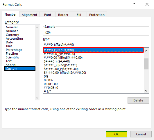
Step 5: Click the OK button, and you can see the negative numbers under parentheses as well as with the text color red. See the screenshot below:
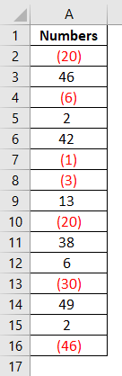
This is how we can represent negative numbers in Excel so that your data read nicely and simply.
Example #4 – Convert the Negative Numbers into Positive
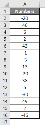
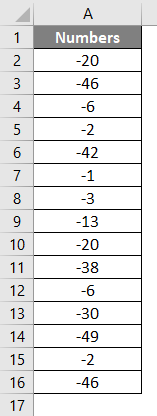
It becomes extremely important in some cases where you need to convert the negative values into positive ones. Follow the steps below to convert negative numbers into positives. Suppose we have a set of negative numbers as shown below:
We have a function in Excel named ABS, which can convert negative numbers into positives. We will use the same for conversion.
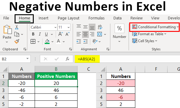
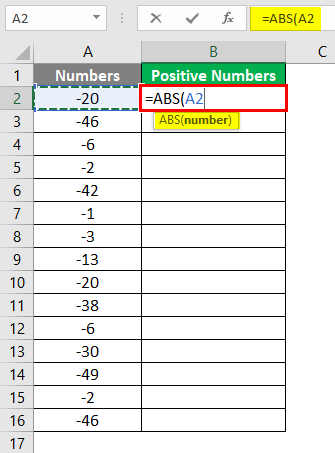
Step 1: In cell B2, initiate the ABS function by typing =ABS(
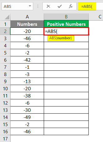
Step 2: Now, use the reference as A2 inside this function. A2 contains the value which we wanted to convert into a positive number.
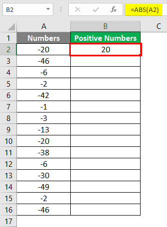
Step 3: Close the parentheses to complete the formula and press Enter key to see the result. The number is converted into a positive number, as shown in the screenshot below under cell B2.
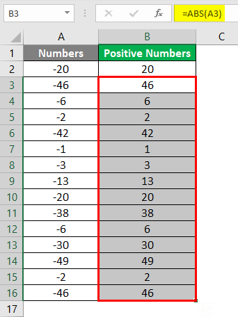
Step 4: Drag the formula across the remaining cells under column B, and you can see the negatives converted into positives.
This is how we can deal with the negative numbers under Excel. Let’s wrap things up with some points to be remembered:
Things to Remember
- While using Conditional Formatting to represent the negative numbers, you need to be very cautious as it is volatile in nature, and any change in numbers will cause it to reassess the condition and apply the formatting again.
- While applying custom formatting, you can also add different colors to the text. Not all colors are available for text formatting. The ones which can be used are primary colors such as Black, Red, Blue, yellow, green, etc.
Recommended Articles
This has been a guide to Negative Numbers in Excel. We discuss Using Negative Numbers in Excel, practical examples, and a downloadable Excel template. You can also go through our other suggested articles –
