Excel FILTER Function

What is an Excel FILTER Function?

We can use the Excel FILTER function to display specific data from a table or array of data by defining certain criteria.

For example, imagine you are organizing an event and have a guest list with 100+ names, and you only want to see the names of guests who have confirmed their attendance (RSVP). You can simply use Excel’s FILTER function for this.

Are you wondering why you need the FILTER function when there is the Auto Filter option? Here’s why.

Imagine you apply Auto Filter to your data and later decide to make some changes. You make some changes, but to your disappointment, the new data is not filtering properly. Why? Because Auto Filter does not automatically update when you modify your data. It means you will have to go through the hassle of cleaning up and reapplying the filter.

So, the solution lies in the Excel FILTER function. Unlike Auto Filter, it effortlessly adjusts to any changes you make to your data. So, no more manual updates or headaches – just smooth, automatic filtering every time you modify your dataset.

Table of Contents

• Definition
• Syntax
• How to Use?
• Examples (with Template)
  • Example #1: Basic Filtering
  • Example #2: Filtering with Multiple Criteria
  • Example #3: Filtering Multiple Criteria with OR Logic
  • Example #4: Filtering Based on Date Ranges
  • Example #5: Filtering Based on Text Criteria
  • Example #6: Filtering Out Blanks
• Errors (with Solutions)

Excel FILTER Function Syntax

This is the syntax for Excel’s FILTER function:

=FILTER(array, include, [if_empty])

• You must add the range of the cells from which you want to filter in the “array”
• The “include” argument represents the criteria or conditions that help the function find the data that you are looking for.
• [If_empty] is an optional argument where you can specify the value to return if no results meet the filtering criteria. If omitted, Excel returns #CALC!

How to Use Excel FILTER Function?

Here is a simple example to illustrate how to use the FILTER function:

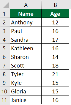
Suppose you have a dataset with names in column A and corresponding ages in column B. You want to filter out the names of people older than 18.

Given:

Here are the steps to achieve this:
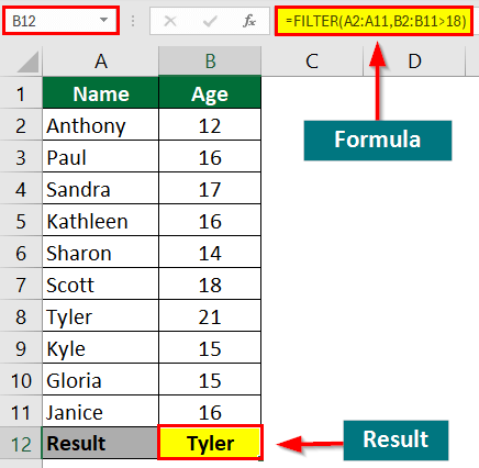
Step 1: Select a cell to display the result. In our example, we choose cell B12.
Step 2: Enter the below FILTER function in cell B12 and hit “Enter”: =FILTER(A2:A11,B2:B11>18)

Result: Here’s how the formula works:
This formula returns the names from column A (A2:A11) where the corresponding age in column B (B2:B11) is greater than 18 (>18).
In this example, Tyler’s age is more than 18.

Excel FILTER Function Examples

Here are some Excel FILTER function examples.

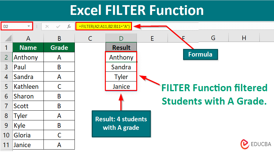
Example #1: Basic Filtering

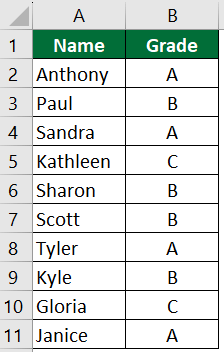
Suppose you add 10 names in the A column and their corresponding grades in column B. You want to filter only the rows where students have scored an A grade.

Given:

Solution:

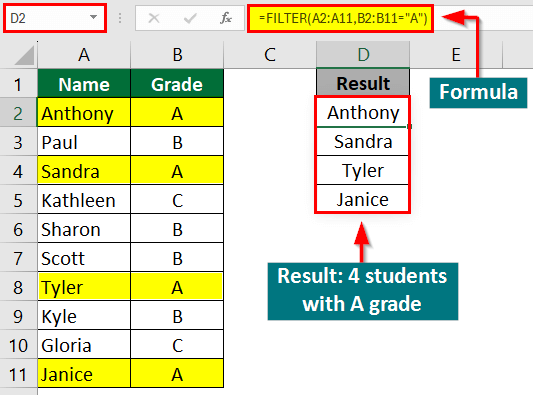
Step 1: Select the cell “D2” where you want the filtered result to appear.
Step 2: Enter the FILTER function in cell “D2” and hit “Enter”:
=FILTER(A2:A11,B2:B11=”A”)

Result:

Anthony, Sandra, Tyler, and Janice scored an “A” grade.

Example #2: Filtering with Multiple Criteria

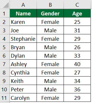
Suppose you want to identify females who are over 30 years old. Let us find out how to find that using the Excel FILTER function.

Solution:

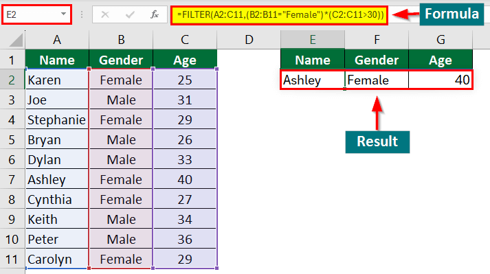
Step 1: Select the cell “E2” where you want the result to appear.
Step 2: Enter the FILTER function in cell “E2” and hit “Enter”:
=FILTER(A2:C11,(B2:B11=”Female”)*(C2:C11>30))

Result:

This filters the dataset to extract only the rows where the individual is female and over 30 years old.
As a result, Ashley is the only female over 30 years old.

Example #3: Filtering Multiple Criteria with OR Logic

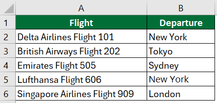
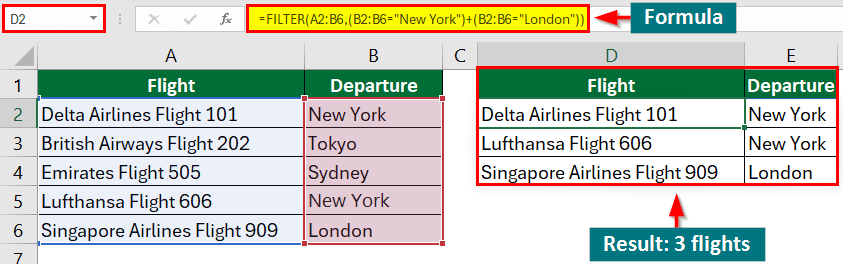
Suppose you have a flight dataset containing flight names and departure locations. You want to filter out flights that either depart from “New York” or from “London”. Here is how you can do it.

Given:

Solution:

Step 1: Select the cell “D2” where you want the result to appear.
Step 2: Enter the below FILTER function in cell “D2” and hit “Enter”:
=FILTER(A2:B6,(B2:B6=”New York”)+(B2:B6=”London”))

Result:

There are 3 flights that depart from either “New York” or “London”.

Example #4: Filtering Based on Date Ranges

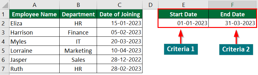
Suppose you have a dataset containing employee names, departments, and their respective joining dates. You need to identify individuals who joined between January 1, 2023, and March 31, 2023. Let’s see how to find them using the Excel FILTER function.

Given:

We will create another table for our criteria. We will set the start date in “E2” (criteria 1) and the end date in “F2”(criteria 2).

Solution:

Add the headings for the filtered data, i.e., Employee Name, Department, and Date of Joining.
Step 1: Select the cell “E5” where you want the result to appear.
Step 2: Enter the FILTER function in cell “E5” and hit “Enter”:
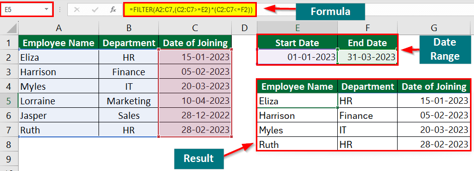
=FILTER(A2:C7,(C2:C7>=E2)*(C2:C7<=F2))

Result:

We can see that 4 employees joined between January 1, 2023, and March 31, 2023, i.e., Eliza, Harrison, Myles, and Ruth.

Example #5: Filtering Based on Text Criteria

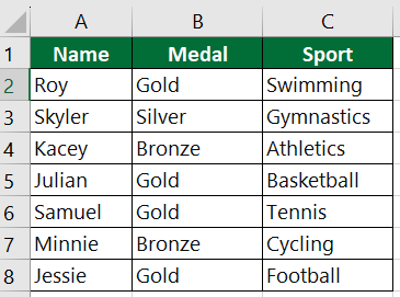
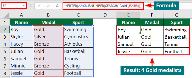
Suppose you have a sports dataset in Excel that includes athlete names, the medals they received, and the sports in which they obtained those medals.
You want to filter the data to show only rows where the text in column B contains the word “Gold.” Let’s see how to do that using the Excel FILTER function.

Given:

Solution:

Step 1: Select the cell “E2” where you want the result to appear.
Step 2: Enter the below FILTER function in cell “E2” and hit “Enter”:
=FILTER(A2:C8,ISNUMBER(SEARCH(“Gold”,B2:B8)))

Result:

We can see that there are 4 gold medalists from the list.

Example #6: Filtering Out Blanks

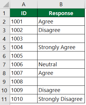
Suppose you have a survey dataset comprising the ID numbers of some individuals and their corresponding responses. A blank response indicates that the individual has not completed the survey. We want to extract only the IDs of those who have responded to the survey. Let’s see how to do that.

Given:

Solution:

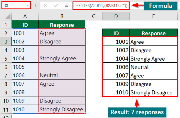
Step 1: Select the cell “D3” where you want the result to appear.
Step 2: Enter the FILTER function in cell “D3” and hit “Enter”:
=FILTER(A2:B11,(B2:B11<>””))

Result:

We can see that we have received 7 responses out of 10.

Excel FILTER Function Errors

If your Excel FILTER function results in an error, it could be due to several reasons. Here are some common errors you might encounter:

1. #VALUE! Error

Excel will return this error if you try to filter a range, but one of the criteria is a text string instead of a number.

To solve this: Double-check the arguments you provide to the FILTER function. For example, ensure that the criteria for numbers are indeed numerical values and that the criteria for text are strings.

2. #SPILL! Error

The FILTER function requires available space to add data into, meaning it needs enough empty cells below and to the right to display all the filtered results. If there is not enough space, Excel will return this error.

To solve this: Ensure there are enough empty cells where you enter the FILTER function. If necessary, adjust the layout of your worksheet to allow for more space.

3. #CALC! Error

This error occurs when Excel cannot complete the calculation due to reasons such as circular references (formulas that directly or indirectly refer to their own cell), insufficient memory, or other calculation-related issues.

To solve this: Check for circular references within your spreadsheet and resolve them or enable “Iterative calculations”. If the error persists, try breaking down your formula into smaller parts to identify where the calculation issue lies.

4. #REF! Error

Excel will return this error if the array or range specified contains errors or is invalid.

To solve this: Check the range or array you specified to ensure it contains valid data. Look for any cells within the range that might contain errors and correct them if necessary.

5. #NAME? Error

This error occurs when Excel cannot recognize one of the functions or names within the FILTER function. It could be a misspelling or a function that does not exist in your version of Excel.

To solve this: Double-check the spelling of all functions and named ranges within the function. Ensure that your version of Excel supports the functions you are using.

6. #N/A error

This error can occur if Excel cannot find any data that matches the filtering conditions.

To solve this: Review and adjust the filtering criteria if necessary to find matches within your dataset. Also, check the data range to see any inconsistencies or issues causing the lack of matching results.

Frequently Asked Questions (FAQs)

Q1. What type of criteria can I use with the FILTER function?
Answer: You can use various types of criteria with the FILTER function, including numerical comparisons (>, <, =), text comparisons (contains, begins with, ends with), logical conditions (AND, OR, NOT), and more.

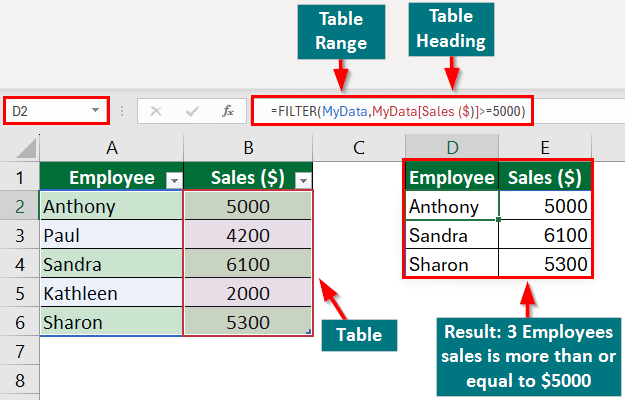
Q2. Can I use the FILTER function with Excel tables?
Answer: Yes, you can use the FILTER function with Excel tables. When using a table as the data range, you can refer to the table columns by their headers in the formula.

Q3. In which version of Excel is the FILTER function available?
Answer: Excel introduced the FILTER function in Excel 365, followed by inclusion in Excel 2019 and Excel 2016 for Office 365 subscribers. Earlier versions of Excel, like Excel 2013 and prior, do not support this function.

Q4. Can I nest the FILTER function within other functions?
Answer: Yes, we can nest the FILTER function within other functions to perform more complex filtering and calculations. For instance, you might use it within functions like SUM, AVERAGE, MAX, MIN, and others to operate on the filtered data set.

Recommended Articles

This article is a guide to the Excel FILTER function, where we discuss how to use the FILTER function in Excel using several examples and provide a downloadable template, too. To learn about more Excel functions, read our suggested articles,

1. Advanced Excel Formulas and Functions
2. Address Excel Function
3. Sorting in Excel
4. Excel Flash Fill