Updated August 21, 2023
Introduction to Bullet Points in Excel
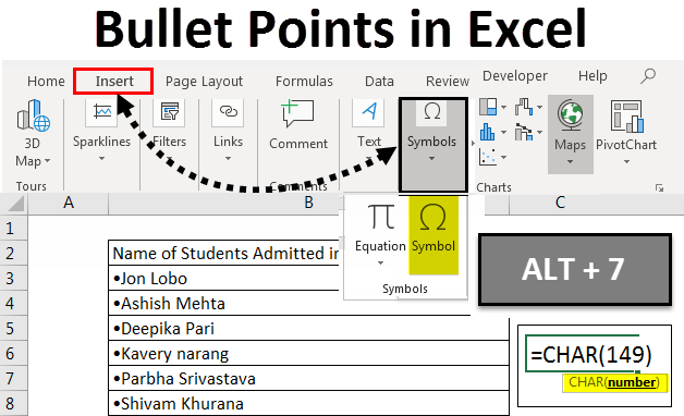
Microsoft Excel is more about numbers and reports. Sometimes you need to present some information in points in your report, and you can do it by adding bullet points in Excel.
There are 6 different ways to use it. But the major drawback is that creating the bulleted list in Excel isn’t as straightforward as in Word documents as there is no direct button for adding bullets on the ribbon in Excel. But that doesn’t mean that we can’t add bullets in Excel.
How to Add Bullet Points in Excel?
As discussed above, we will show you the steps below to add bullet points in Excel by using 6 Different ways with some examples.
Example #1 – Using Keyboard Shortcuts
The Simplest and quickest way to add the bullet symbol into the Excel sheet cell is by using keyboard shortcuts.
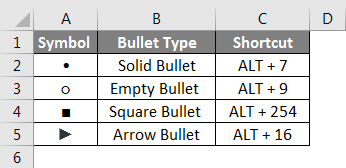
- Alt + 7 to insert a Solid Bullet.

- Alt +9 to insert an Empty Bullet.

- Alt +254 for the Square Bullet.

- Alt +16 For Arrow Bullet

You must use your numeric keypad to use the numbers key with Alt+tab. You may need to use different shortcuts if you are working on a laptop.
Users can use square or arrow bullet points instead of the usual solid and empty bullets to add some fancy bullet points.
Example #2 – Using the Symbol Dial Box
You can use Symbol Dial Box if you don’t have a number pad on your keyboard or forget Keyboard shortcuts.
We will show you this step by step and with an example.
- Open an Excel Sheet.
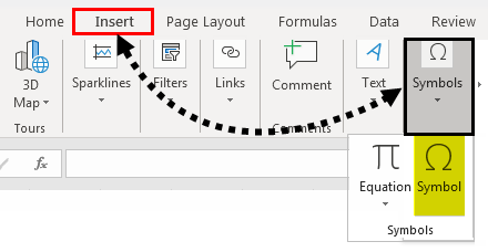
- Go to the Insert tab.
- Select Symbols >Symbol under the Insert Tab.
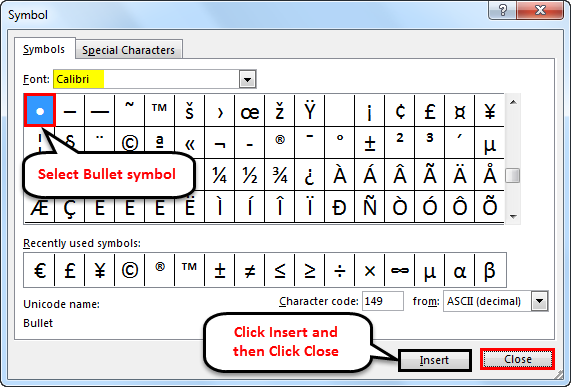
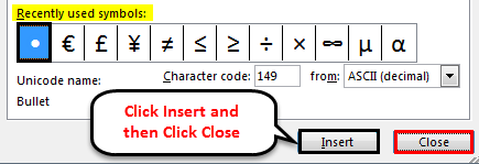
- After Selecting the symbol, a dialog box will open; Font Calibri will automatically get selected in the Font Dropdown, but you can select any font, select the bullet symbol you want to use, click Insert, and then click Close.
- You can copy-paste the symbol to the next Row or Column.
So, in the above steps, it is shown how to insert by using the symbol tab under the Insert tab, and now let’s take a simple example.
We need to show the number of children admitted to School in 2019, and we want to show this data in the Excel file.
- Open the Excel File.
- Go to Insert Tab, and Select Symbol under Insert Tab.
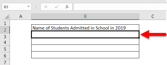
- So, in the file, we have created the heading “Name of Students Admitted in School in 2019.”
- So before adding the names under it, we will add bullet points before the name as we want to show our data in Bullet Points. First, we will select the B3 cell.
- We will click on the Insert tab and select Symbol; a dialog box will appear after selecting the symbol. Next, we will select the Bullet symbol and select Insert.
- The bullet will insert in a column, and you can update the student’s name.
- A bullet is inserted in Column B3 & now you can type a student’s name. This way, you can add a bullet in another column and update the name, or you can copy-paste by using (CTRL+C) for copying and (CTRL +V) for pasting the bullet in other columns till where you want to update the data.

- So this way, the bullets are added using the Symbol tab. For any List or Worksheet, you can use it in a similar way.
Example #3 – Using a Function
It is useful when you want to add bullets to multiple cells at a time to use the CHAR function. It takes a character code and displays the character corresponding to it in the cell. We will show you an example of how to use this function.
- Open an Excel Sheet.
- Let’s say we have a list of fruits in Column A of the Excel sheet.
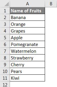
- We will convert the above list of fruits to the bulleted list in Column B using CHAR Formula.
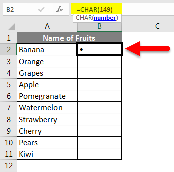
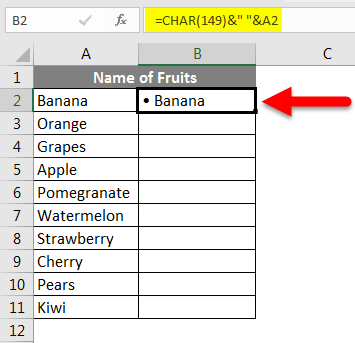
In B2, we will put the formula (=CHAR(149)), adding a bullet to the column.
- If you want to add the name of the fruit after the bullet, you can type this formula (=CHAR (149)&” “&A2). This Formula concatenates a solid bulled character, one space, and the value of the referenced cell(A2).
- This method is useful if you list items in one column without the bullet. To copy the formula in other columns, drag the AutoFill box in the lower-right corner of the cell and scroll it down until you want to fill your data, as shown below.
Example #4 – Using Custom Formatting
Custom Number Formatting is an amazing technique useful in a long Bulleted list as it adds the bullets to your list items faster and is useful when you don’t have a number pad.
Let’s discuss this feature with an example.
- Open an Excel File.
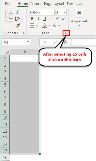
- We will select 15 cells in the Excel sheet in column A.
- After Selecting the cells, we will press (CTRL+1) to open the Format Cell dialog box, or you can go to the Home tab and click the small icon below to open the dialog box.
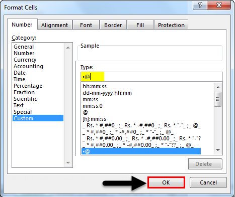
- When the dialog box appears, we will go to the Number tab and select Custom from the below list.
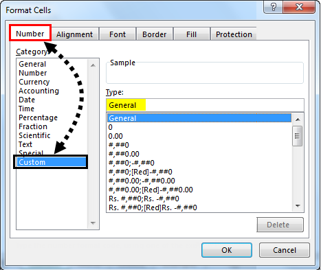
- After Selecting Custom, a General Field will appear after Selecting Custom, as shown in the screenshot above. This field allows you to specify the format of the selected cells, which we selected in our second step (15 cells) from Column A1 to A15.
- Now we will add bullet points by putting Bullet Symbol(you can copy the symbol from anywhere) and paste it in the type box, space, and then @ character, and Click OK.
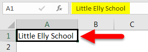
- If you type “Little Elly School” in the A1 Cell and hit Enter, it will automatically come with the bullet point. If you check the formula bar, the value remains the same, which was only Little Elly School.
- Similar formatting will be applied for the 15 cells we selected in the starting & whatever you type in these cells, they will come up with bullet points.
- We have added the data on all 15 cells with the school names using the same function. It will all come up with the bullet points in the Excel worksheet.

Example #5 – By copying it From Microsoft Word
This feature is very simple and easy as we all know that we have the Bullet Feature in Word, so we can add our list of items in word with Bullet Points, copy the data from Word, and paste it into Excel by double-clicking the cell of a column.
- Open the Microsoft Word Document.
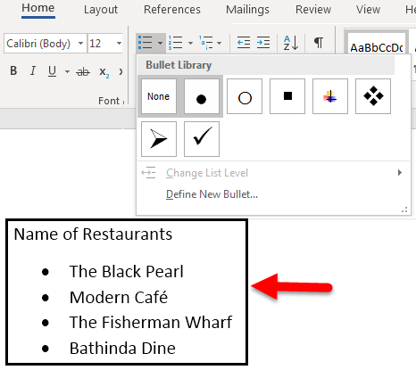
- Select the Bullet Point feature in Word and type the data you want to update in Excel File. Then, copy the data by using CTRL+ C.
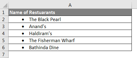
- Open the Excel File and Paste the data by double-clicking on the cell (or press F2) and then Press (CTRL+V) in the Excel file. The Data copied from Word will be pasted into the Excel sheet.
Example #6 – Entering Multiple Bullets in One Cell (ALT + ENTER)
Suppose you want to enter multiple bullet points in one cell. You can simply do this by following the below steps.
- Double click on the cell or press F2.
- Now insert the bullet point by following the above methods and enter the text you want.
- After entering the text, press ALT + Enter

- This will take you to another line in the same cell.
- Now you can add bullets again and enter the text.
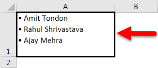
For example, Look at the below screenshot, where I have entered multiple bullet points line items in a cell.
Things to Remember
- Bullet Point helps Clarify Writing as it avoids information in long texts and adds just the brief with quick information, but you should use it Wisely and in Limit.
- Bulleted Lists should be arranged in an order that makes them as efficient as possible.
- Bullets are designed for clarity, not confusion, so you should avoid using more bullets and sub-bullets.
- Never have only one bullet. However, if you have a list of information, these bullet points are useful.
Recommended Articles
This has been a guide to Bullet Points in Excel. Here we discussed How to add Bullet Points with different Excel methods, practical examples, and a downloadable Excel template. You can also go through our other suggested articles –
