Updated June 8, 2023
Excel COUNTIF Example (Table of Contents)
Excel COUNTIF Examples
Excel COUNTIF Example counts the cells that meet certain criteria or conditions. It can count cells that match specific criteria with text, numbers or dates. By referring to some COUNTIF examples in Excel, you can understand the use and implantation of the COUNTIF Function.
Syntax of COUNTIF Example in Excel
The Syntax of the COUNTIF Function includes 2 parameters. Before we apply COUNTIF, first let’s see the syntax of the COUNTIF Function in Excel, as shown below;
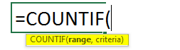
Range = The range we must select from where we will get the count.
Criteria = Criteria should be any exact word or number we need to count.
The return value of COUNTIF in Excel is a positive number. The value can be zero or non-zero.
How to implement Excel COUNTIF Examples?
Using the COUNTIF Function in Excel is very easy. Let’s understand the working of the COUNTIF Function in Excel by the examples below.
Excel COUNTIF Example – Illustration #1
The COUNTIF function in Excel is used for counting cell content in selected range data. The selected cells may contain numbers or text. Here we have a list of some products which are repeated multiple times. Now we need to check how many times a product gets repeated.
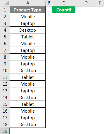
As we can see in the above screenshot. We have some product types, and besides that, we have chosen a cell for counting cells of a specific product type.
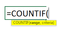
For applying the COUNTIF Function example, go to the cell where we need to see the output and type the “=” (Equal) sign to enable all the inbuilt functions of Excel. Now type COUNTIF and select it.
Range = Select the range as A2:A18.
Criteria = For text, let’s select the criteria as Mobile in inverted commas (“); it is a text.
As we see below the screenshot, how our applied COUNTIF final formula will look like. Blue colored cells are our range value, and in inverted commas, Mobile is our criteria to be calculated.
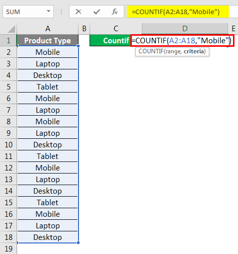
Once we press the Enter key, we will get the applied formula as shown below.
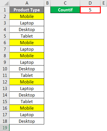
As we can see, the count of product type Mobile is coming as 5, which is also highlighted in yellow in the above screenshot.
We can test different criteria to check the correctness of the applied formula.
Excel COUNTIF Example – Illustration #2
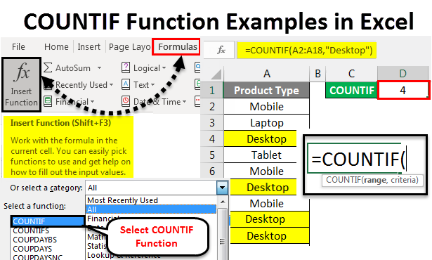
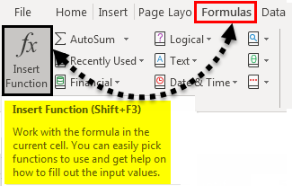
There is one more method of applying the COUNTIF Function in Excel. For this, put the cursor on the cell where we need to apply COUNTIF and then go to the Formula menu tab and click on Insert Function, as shown in the below screenshot.
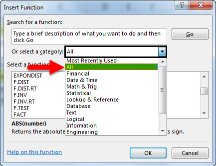
Once we click on it, we will get the Insert Function box with the Excel list of inbuilt functions, as shown below. From the tab, select a category, and choose All to get the list of all functions.
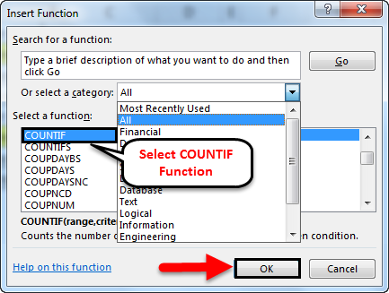
And from the Select a function box, select COUNTIF and click OK. Or type COUNTIF or a keyword related to this and find related functions in the Search for a function box.
After that, we will see the function argument box, where we need to select the same range as we did in Illustration #1 but with different criteria as Desktop and click on OK.
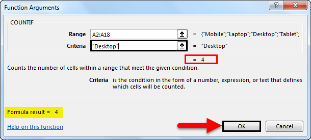
If the formula is correct, we will see it resulting in the Function arguments box, as highlighted. After that, we will get the result in the output cell, as shown below.
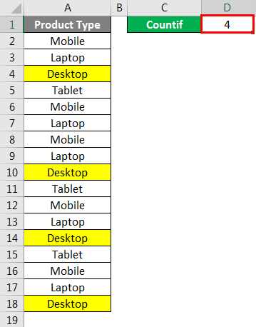
As we can see in the above screenshot, the Desktop count is 4. Which are also highlighted in yellow color in the above screenshot?
For this process also, we can test different criteria to check the correctness of the applied formula.
This is how the COUNTIF function is used to calculate the numbers or words that are repeated multiple times. This is quite helpful where the data is so huge that we cannot apply filters.
Excel COUNTIF Example – Illustration #3
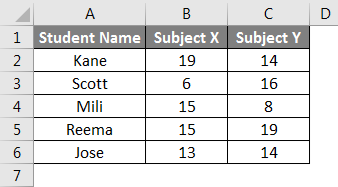
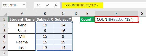
Let’s see one more example of the COUNTIF Function in Excel. We have a list of some students where student marks of Subject X and Subject Y are mentioned in columns B and C. Now with the help of the COUNTIF Function Example, we will see how many students got 19 Marks out of 20.
For this, go to the cell where we need to see the output. Type = (Equal) sign and search for the COUNTIF function and select it as shown below.
Now select the range. Here, as we have two columns where we can count the values, we will select columns B and C from cell B2 to B6. By this, we will be covering the B2 to C6 cell range. For the criteria, type 19 in inverted commas, as shown below.
After that, press the Enter key to apply the formula, as shown below.
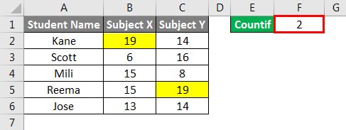
As we can see in the above screenshot, the COUNTIF function counted that only 2 students got marks that are 19 in any subject.
Here, by applying COUNTIF functions where the range is more than one column, the function checks the criteria in the selected range and gives the result. As per the above marks, Kane and Reema are students who got 19 marks in one of the subjects. There could be cases where we could get 19 marks against a single entry irrespective of the range selected, but the output will be the combined result of data available in the complete selected range.
Things to Remember
- The second parameter in the formula “Criteria” is case-insensitive.
- As a result, only the values that meet the criteria will be returned.
- If the wildcard characters are to be used as they are in the criteria, the tilde operator must precede them, i.e., ‘~? ‘, ‘*’.
Recommended Articles
This has been a guide to Examples of the COUNTIF Function in Excel. Here we discuss how to use COUNTIF Example in Excel, practical illustrations, and a downloadable Excel template. You can also go through our other suggested articles –
