What is P-Value in Excel?
The p-value in Excel is a statistical measure that checks if the correlation between the two data groups is caused by important factors or just by coincidence. It plays a vital role in analyzing real-world issues in areas like medicine, economics, and human study.
Statisticians and researchers commonly use the p-value when they want to analyze two data groups. They start by considering a null hypothesis, which assumes there is no relationship between the two data groups. This serves as their initial assumption for the experiment. Then they conduct various statistical tests, including the p-value, and interpret the results. For instance, if the p-value is greater than the significance level (α) of 0.05 (5%), it suggests that the two data groups are indeed related. Therefore, the initial assumption of the null hypothesis was incorrect. Conversely, if the p-value is less than 0.05 (5%), it indicates that the two data groups are unrelated, supporting the initial null hypothesis assumption.
Statisticians can use Excel to quickly and easily calculate the p-value. Although Microsoft does not have any specific or direct formula for p-value in Excel, we can use functions like T.TEST and T.DIST for the calculation. Moreover, there is another method: Analysis ToolPak, that basically simplifies the T.TEST function for us.
Table of Contents
How to Calculate P-Value in Excel?
In this section, we will see how to calculate P-Value in Excel using examples. Here are the three different ways or functions that we will use:
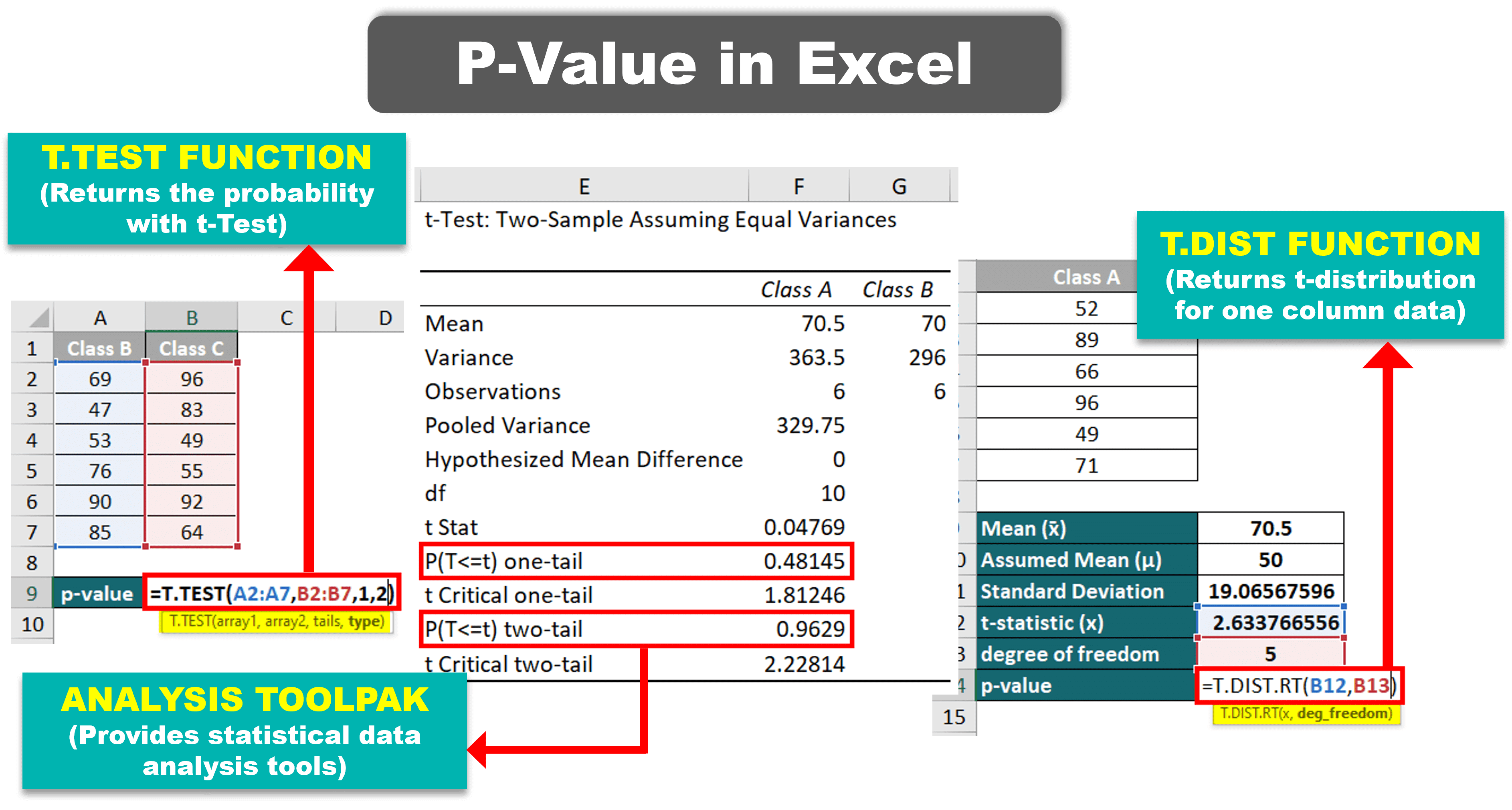
- T.TEST Function
- Analysis ToolPak
- T.DIST Function
1. T.TEST Function
Purpose: We can use the T.TEST Function to calculate the p-value in Excel by directly adding the data ranges to the function.
Syntax:
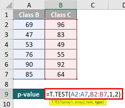
=T.TEST(range1, range2, tails, type)
In this syntax:
- range1: Cell range of the first data set
- range2: Cell range of the second data set
- tails: Specifies if the test is one-tailed (1) or two-tailed (2).
- type: It determines the type of t-test. [1 for before and after comparison, 2 for an equal number of data in all columns, and 3 for an unequal number of observations in all the data.]
Example:
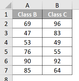
Let us compare the scores of students from Class B and Class C to check if Class C students have higher scores than Class B students. First, we need to assume the null and alternate hypotheses for this test.
Null Hypothesis (H0): There is no difference in the scores of both divisions.
Alternate Hypothesis (H1): Class C students have higher scores.
We will calculate the p-value to determine if we should accept or reject the null hypothesis.
Consider the following data:
Solution:
Step 1: Select cell B9 and write the below formula:
Step 2: Press “Enter,” and Excel will calculate the p-value as 0.38692 in cell B9.
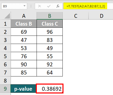
Result:
| P-Value: | 0.38692 (39% approx) |
| Significance level (α): | 0.05 (5%) |
| Our Analysis: | p-value > α |
| Our Conclusion: |
|
Based on the analysis, we can conclude that the p-value obtained (0.38692, approximately 39%) is higher than the significance level (α) of 0.05 (5%). Therefore, we reject the null hypothesis (H0), which assumes no difference in scores between the students of both classes. Consequently, we accept the alternate hypothesis, which suggests that Class C students have higher test scores than Class B students.
2. Analysis ToolPaK
Purpose: The Analysis ToolPak is an Excel Add-in feature that makes it easier to perform t-tests. By simply inputting the necessary information in a new window, ToolPak automatically calculates and shows the p-value.
Here,
You will have to enter the following:
- Variable 1 Range: Range for the first data column
- Variable 2 Range: Range for the second data column
- Labels: Allows Excel to display the column headings in the output
- Alpha: The standard value for p-value comparison (0.05)
- Output Range: Cell where Excel should display the output.
Example:
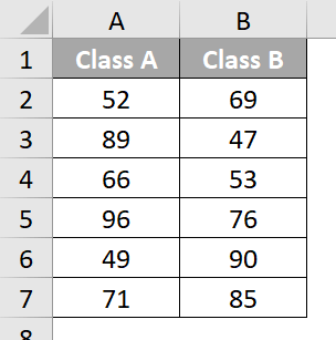
Let us compare the scores of students from Class A and Class B to investigate whether Class A students have higher scores on their exams than students from Class B.
Null Hypothesis (H0): There is no difference in the average scores between both divisions.
Alternate Hypothesis (H1): Class B students have higher average scores.
We want to calculate the p-value to check if our assumption in the null hypothesis is true or false.
Consider the following data:
Solution:
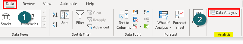
Step 1: Click the “Data Analysis” option from the “Data” Tab.
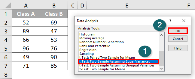
Step 2: A “Data Analysis” dialogue box will open, from which you have to select “t-Test: Two-Sample Assuming Equal Variances”. Then click “OK”.
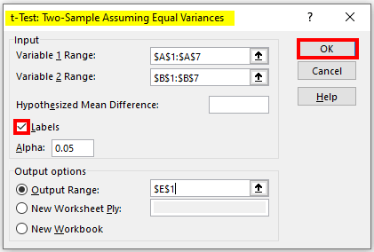
Step 3: Add the necessary information in the dialogue box as shown below:
- Variable 1 Range: A1 to A7
- Variable 2 Range: B1 to B7
- Labels: Tick the checkbox
- Output Range: E1.
After entering the above data, click on “OK”.
Excel will provide a detailed result for the p-value in cells E1 to G14, as shown below:
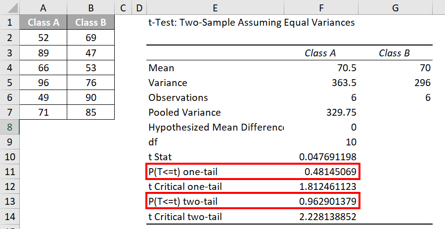
Result:
| One-tailed P-Value: | 0.48 |
| Two-tailed P-Value: | 0.96 |
| Significance level (α): | 0.05 |
| Our Analysis: | p-values > α |
| Our Conclusion: |
|
The tool gives us two p-values: one for a one-tailed t-test and the other for a two-tailed t-test. Both p-values, 0.48 (approximately) and 0.96 (approximately), are greater than the significance level (α) of 0.05 (5%).
As the p-value is higher than 0.05, it indicates that the alternate hypothesis is true, suggesting that Class B students have scored more than Class A students. Therefore, we reject the null hypothesis, which assumes no difference between the average scores of students from both classes.
3. T.DIST Function
Purpose: We can use Excel’s T.DIST Function to calculate the p-value by simply adding the test statistic value and degree of freedom.
Syntax:
= T.DIST.RT(x, degrees_freedom)
In this syntax:
- Rt: It is for calculating one-tailed (one-sided) sample data. There is another variation T.DIST.2T for two-tailed data for comparison between two sets of data.
- x: It is the test statistic value, i.e., the value we want to study
- degrees_freedom: Degrees of freedom for the T-distribution
Example:
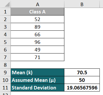
The school headmaster believes that students cannot score above 50 without attending tuition classes, so they plan to start a special class for all students. To investigate this belief, a teacher chooses a random group of 6 students and records their scores in a specific subject. The average score of this group is 70.5, with a standard deviation of 19.06.
We need to calculate the p-value using the t-dist function to see if the headmaster’s assumption (students that do not attend tuition classes cannot score more than 50) is true or not.
Null Hypothesis H(0): Students can score higher than 50 even without attending tuition.
Alternate Hypothesis H(1): Students score lower than 50 if they do not attend tuition.
Consider the following data:
Solution:
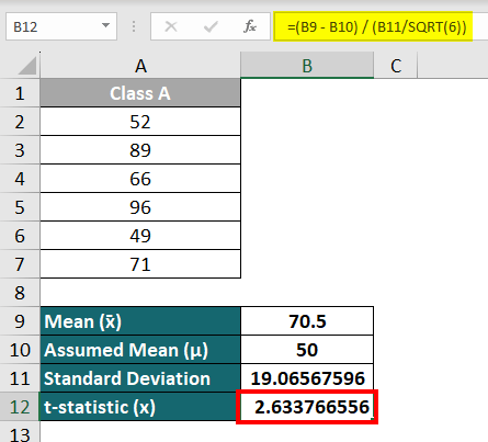
Step 1: Calculate the test statistic value (x) using the following formula,
Test statistic = (x̄ -μ) / (s/√n)
We can write the above formula in the Excel format as follows:
Enter the above formula in cell B12 and press “Enter”. As a result, Excel will show the x value as 2.634 (approx).
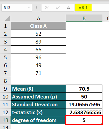
Step 2: Calculate degrees of freedom in cell B13 as follows:
Degree of freedom = No.of observations (n) – 1
= 6 – 1
= 5
Step 3: Now, we will find the p-value in Excel using the T.DIST Function.
- Enter the below formula in the cell B14
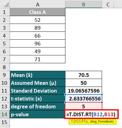
- Press “Enter,” and Excel will display the p-value as 023161286 in cell B14.
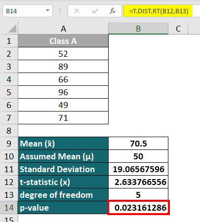
Result:
| P-Value: | 0.02316 (2.3% approx) |
| Significance level (α): | 0.05 (5%) |
| Our Analysis: | p-value < α |
| Our Conclusion: |
|
The T.DIST function returns the p-value as approximately 0.023.
We can see that the p-value of 0.023 (2.3%) is less than the significance value (α) of 0.05 (5%). Therefore, the null hypothesis is correct; the students can score more than 50 without attending tuition. Thus, we accept the null hypothesis.
Things To Remember About P-Value in Excel
- It is important to select the null and the alternate hypothesis carefully.
- Slight variations in the final p-value, even if higher or lower by a few numbers, do not significantly impact the overall analysis.
- The default value for alpha (α) in the Analysis ToolPak is 0.5, but users can modify it according to their needs.
- In a one-tailed test, we compare two data sets to determine if the first dataset is higher than the second. On the other hand, in a two-tailed test, we examine whether the two datasets have any difference at all. In this case, the first dataset can be either smaller or higher than the second, or there may be no difference. The two-tailed test considers all possibilities of the difference without specifying a specific direction.
Note: Tackling advanced topics like p-value, Azure, etc., can be challenging when preparing for IT and Excel certifications. In such situations, having access to dependable study materials and certification resources, like the Microsoft AZ-500 Exam dumps, can be beneficial.
Frequently Asked Questions (FAQs)
Q1. Can the p-value be negative?
Answer: No, the p-value is never negative because it can only have a value between 0 and 1. Therefore, the p-value is always positive.
Q2. What is a strong vs. weak p-value?
Answer: A weak or small p-value is when the p-value is less than 5% (P-Value < 0.05). It means the null hypothesis is true, indicating that there is no difference between datasets. In contrast, a strong or large p-value is when the p-value is more than 5% (P-Value > 0.05). It means the alternate hypothesis is true, suggesting that there is a real difference, and it’s not just by coincidence.
Q3. What causes the p-value to decrease?
Answer: The p-value can decrease due to several reasons:
- Increasing the number of observations in a data set leads to a smaller p-value, enhancing the accuracy and reliability of our estimates.
- If there is a huge difference between both the data ranges, it becomes easily noticeable, and the p-value decreases.
- When the data points are very close to each other, we can clearly see that there is no major difference between the sets. Thus, the p-value will be lower.
Lastly, if we set a higher standard for what we consider significant, it becomes harder to get a small p-value.
Recommended Articles
This has been a guide to P-Value in Excel. Here, we discussed the calculation of P-Value, with practical examples and a downloadable Excel template. You can also go through our other suggested articles –
