Updated May 9, 2023
Definition of Trunc in Excel
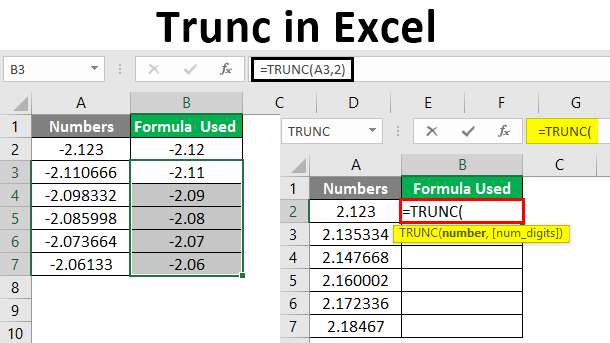
Trunc is also known as the Truncate function in Excel. It is considered one of the mathematical and trigonometrical functions of Excel. The output returned by this function is a numeric value. The syntax for this simple function is =TRUNC( number, number of digits). Out of these two parameters, the first argument is mandatory, and the second argument is optional. The first argument is the input we provide to the function, which is the number to be truncated, and the second argument is the number of digits we want displaying in a decimal value input. Let us discuss what these two arguments are.
How to Use Trunc in Excel?
The Trunc function is similar to the INT function in Excel because both functions give us the result for the integer part of the number. The Trunc function has two arguments where one is mandatory, and one is optional. The mandatory argument is the integer input.
Example #1
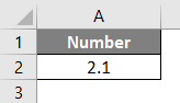
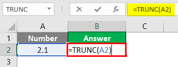
Let us review our basic example to learn how to use Excel’s Trunc or truncate functions. Let’s assume we have a value of 2.1 in cell A1 as shown below:
We have value in cell A2; let us use the function in cell B2 as follows:
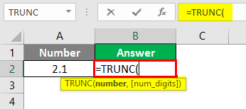
We know that the first argument is mandatory, which is the number we want to truncate, so select cell A2 for the following argument:
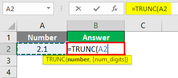
The second argument is optional, which is given when we need to remove a part of the number, which can be a fractional part of the decimal part, so that we can close the parenthesis.
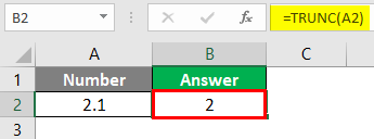
When we press the Enter key, we will have our final result as shown below:
Example #2
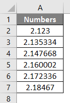
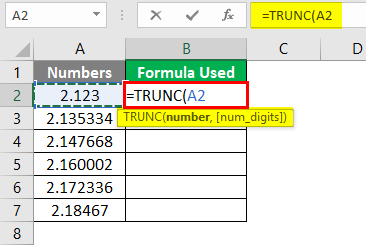
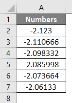
For this example, we have a bunch of numbers that are in decimal parts, and they are positive integers; we will use a truncate function for these numbers as shown below:
Let us use the number of digits to be truncated as 2.
In cell B2, type the following formula shown in the screenshot below.
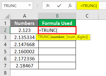
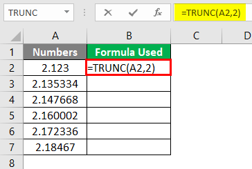
Please select the number from cell A2, as shown in the screenshot below.
Now, after the number, put a comma and type 2 for the number of digits to be truncated, as shown below:
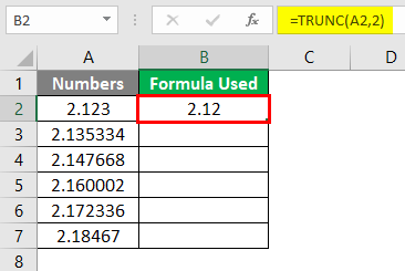
Press Enter Key and see the result.
Copy the formula and drag it to the last cell, as shown below.
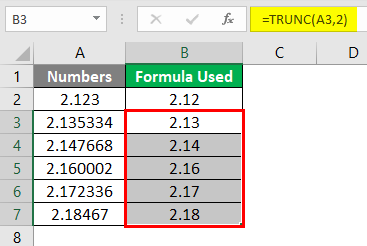
The values in cell B2 are the truncated numbers truncated to the two digits from the original number.
Example #3
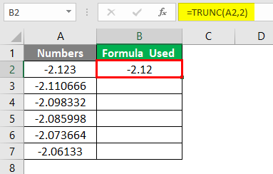
In the previous example, we used positive integers to show how the trunk function works. Now let us see if we will get the same result for the negative integers. We have the following number in cell A2, as shown below.
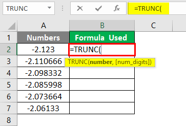
Again let us use the number of digits to be truncated as 2. In cell B2, type the following formula shown in the screenshot below.
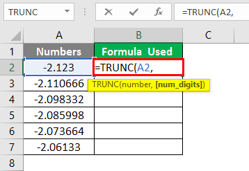
Please select the number from cell A2, as shown in the screenshot below.
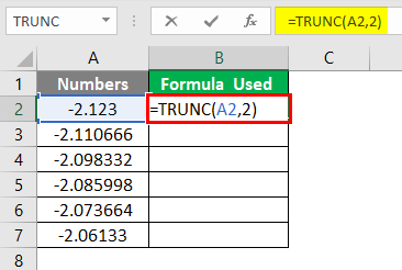
Now, after the number, put a comma and type 2 for the number of digits to be truncated, as shown below:
Press Enter Key and see the result.
Copy the formula and drag it to the last cell, as shown below.
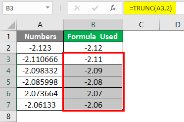
In column B, we have the desired result from the Truncate function.
Example #4
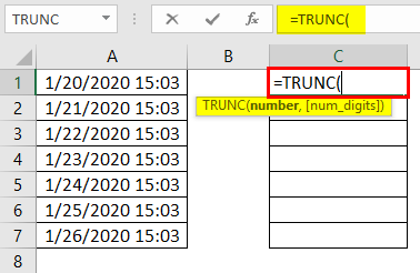
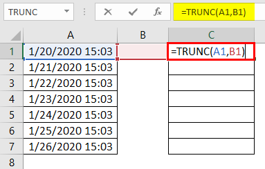
Now there is one example when we get data from some external source, and the date from the source has a timestamp attached. So can we use the Trunc function to extract the date from the timestamp? Let us find out. I have the below dates in the timestamp format.
In cell C1, type the following formula as shown in the screenshot below:
For the number argument, select cell A1.
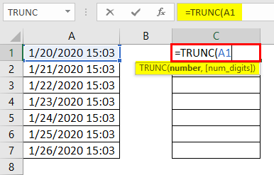
For the number of digits to be truncated, select cell B1; since it is blank, it will be considered 0.
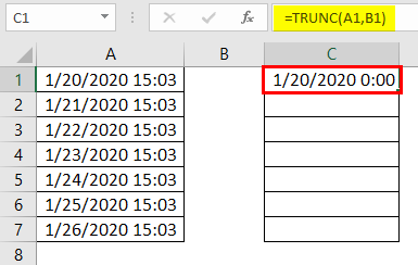
Press Enter Key and see the result.
Copy and drag the formula to cell C7, as shown in the screenshot below.
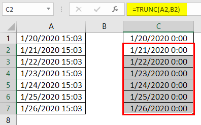
We have successfully extracted the date using the Trunc function from the data.
Things to Remember
- The Trunc function is one of the mathematical and trigonometrical functions of Excel.
- INT and TRUNC functions are similar.
- The values returned by this function are numeric.
- The Trunc function is categorized under the mathematical and trigonometrical functions of Excel. This function returns a number to a specified number of digits. This function gives us a numerical value.
Recommended Articles
This is a guide to Trunc Function in Excel. We discuss using Trunc Function in Excel, practical examples, and a downloadable Excel template here. You can also go through our other related articles –
