Updated May 9, 2023
Excel MINVERSE (Table of Contents)
Definition of Excel MINVERSE
The reciprocal of any square matrix is called the inverse. For a matrix to be invertible, there are two basic conditions to be satisfied:
- The matrix we want to find the inverse needs to be a square matrix. It should have an equal number of rows and columns.
- The determinant of the matrix should not be zero. If it is so, the matrix is said to be non-invertible.
Syntax:
Following is the syntax for the MINVERSE function in Excel, which can be used to compute the inverse of a matrix:
Where,
- Array – This mandatory argument specifies an array of values representing a matrix.
Examples of MINVERSE in Excel
Lets us discuss the MINVERSE in Excel with some examples.
Example #1 – Computing Inverse of a 2X2 Matrix
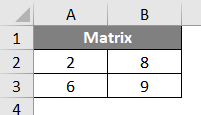
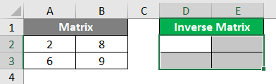
A matrix with two rows and two columns is considered a 2X2 matrix. Suppose we have a 2X2 matrix as shown below:
Well, if you check, this matrix follows both mandatory conditions for a matrix to be invertible.
- Since it has two rows and two columns, it is a square matrix
- The determinant of a matrix can be computed as “ad-bc”. Here a=2, b=8, c=6 and d=9. Thus ad-bc results in (2*9)-(6*8) = 18-48 = 30 which is non-zero.
We will store the inverse of this matrix in columns D and E spread along with the cells D2:E3. Hence, it is clear that the given matrix is invertible. See the screenshot below:
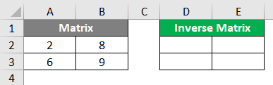
Step 1: Select all the cells under the Inverse Matrix section from D2 to E3 as shown below:
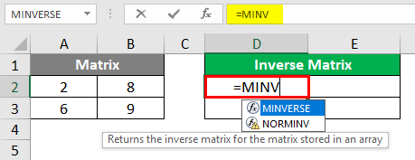
Step 2: In the active cell (cell D2), start typing =MINV, and you’ll see all the formulae associated with that keyword. Out of those, select the MINVERSE function by double-clicking on it to find out the inverse of a given 2X2 matrix.
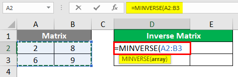
Step 3: The mandatory argument needed for this function is an array. Use the original matrix cells containing values as an array for this one (i.e., A2:B3 in our case). Note that this is a mandatory argument for the MINVERSE function. See the screenshot below:
Step 4: As discussed earlier, MINVERSE is compatible with arrays only. Thus, instead of pressing the Enter key, we need to press Ctrl + Shift + Enter button. A sequence of keys that converts the formula into an array formula. Once you hit the button, you can see the inverse of a given matrix in D2:E3, as shown below:
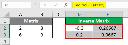
Notice the curly braces within which the entire formula is enclosed. These indicate that the formula works as an array formula over the given range.
Example #2 – Computing Inverse of a 4X4 Matrix
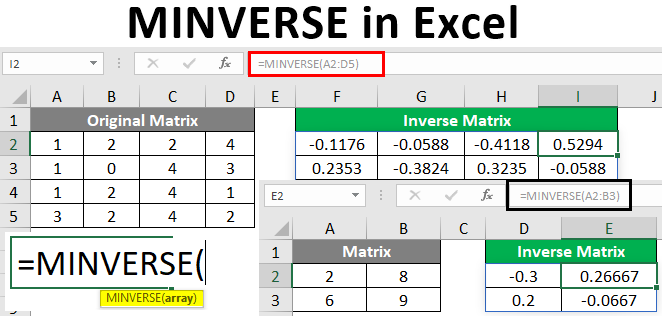
Let us now consider a 4X4 square matrix, for which we need to compute the inverse.
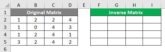
Incidentally, across cells F2 to I5, we will store the inverse of our original matrix. Follow the steps below to compute the inverse of the original matrix spread along with cells A2 to D5.
Step 1: Select all the cells for the Inverse matrix varying across F2 to I5, as shown in the screenshot below:
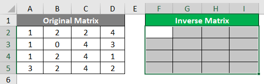
Here is an interesting task: the Original Matrix is invertible (which means it should satisfy both conditions). Could you check if the determinant of this matrix is non-zero? (It is, but check with manual calculations on your own.
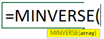
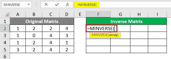
Step 2: Inactive cell, i.e., cell F2, initialize the formula for the inverse of a matrix by typing =MINVERSE(
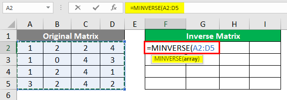
Step 3: Use the Original Matrix cells spread across A2: D5 as a mandatory array argument to this formula. Since that is the matrix array, we wanted to find out the inverse.
Step 4: Close the parentheses to complete the formula and Press Ctrl + Shift + Enter key to convert this formula into an array formula. Remember, this formula is developed in a way compatible with arrays only.
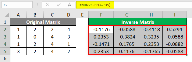
As soon as you press the keyboard strokes, you’ll see the output below under the Inverse Matrix section.
That is the Inverse matrix of our original matrix spread across A2: D5. Look at curly braces, which indicate that the formula is converted into an array. This is how we can use the Excel MINVERSE function to compute the inverse matrix of any square matrix with a non-zero determinant. This article ends here; let’s wrap up some points to be remembered:
Conclusion
- MINVERSE function in Excel is categorized under the “Math and Trigonometry” section within Formulas.
- This function helps us find the inverse of a square matrix with a non-zero determinant value. Note that MINVERSE is an array function developed in a way that can only be compatible with arrays.
Things to Remember
- A matrix for which you expect to compute an inverse matrix must be square. Meaning it should have an equal number of rows and columns.
- If the determinant of the original matrix is zero, you’ll get #NUM! Error. Such a matrix is called a Singular Matrix.
- If some extra cells are selected under the resulting matrix, which is not a part of the matrix, you’ll get the #N/A error.
- The matrix should contain numeric values only. If any blank cell or text values are under the given matrix, you’ll face #VALUE! Error while computing an inverse of the same.
- Array arguments can also be provided as array constants such as {2, 3, 4, 5}. In which the rows and column arguments are separated by semicolons within the curly braces.
Recommended Articles
This is a guide to MINVERSE in Excel. Here we discuss How to use MINVERSE in Excel, practical examples, and a downloadable Excel template. You can also go through our other suggested articles –
