Updated August 11, 2023
Filter Column in Excel
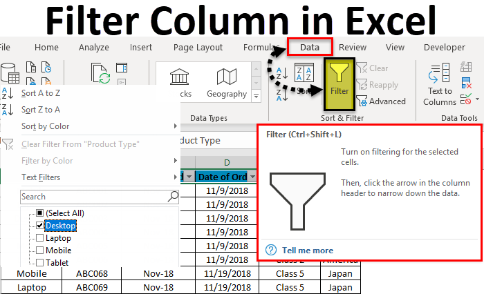
Filter Column in Excel are used for filtering the data by selecting the data type in the filter dropdown. Using a filter, we can make out the data we want to see or on which we need to work.
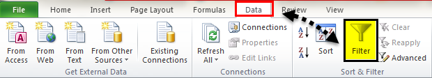
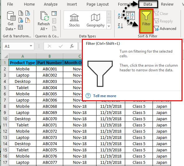
To access/apply a filter in any column of excel, go to the Data menu tab; under Sort & Filter, we will find the Filter option.
How to Filter a Column in Excel?
Filtering a column in Excel is a very simple and easy task. Let’s understand how to filter a column in Excel with an example.
We have some sample data tables in excel, where we will apply the filter in columns. Below is the screenshot of a data set, which has multiple columns and multiple rows with various data sets.
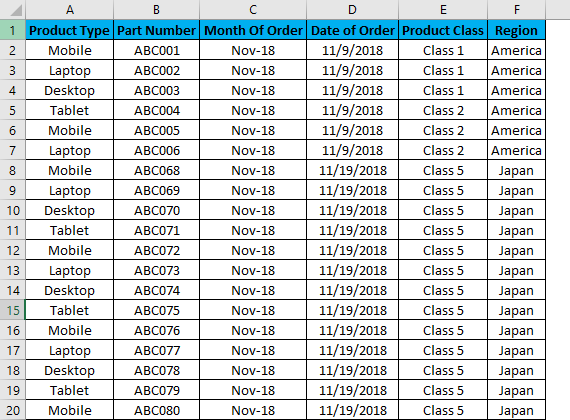
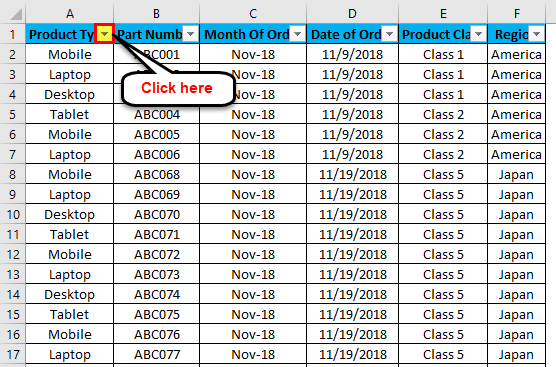
For applying Excel Column Filter, select the top row first, and the filter will be applied to the selected row only, as shown below. Sometimes when we work for a large data set and select the filter directly, the current look of the sheet can be applied.
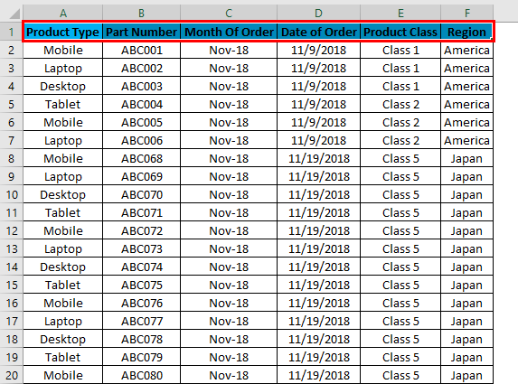
As we can see in the above screenshot, row 1 is selected and ready to apply the filters.
Now for applying filters, go to the Data menu, and under Sort & Filters, select Filters.
Once we click Filters, we can see the filters will be applied in the selected row, as shown in the screenshot below.
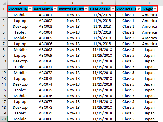
The top row 1 now has the dropdown. This drop-down is those things by which we can filter the data as per our needs.
To open the drop-down option in an applied filter, click on the down arrow (as shown below) or go to any column top and press Alt + Down.
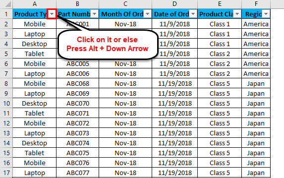
A drop-down menu will appear, as shown in the below screenshot.
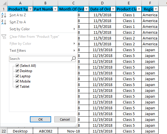
As we can see in the above screenshot, a few filter options are provided by Microsoft.
- Sort A to Z / Sort Oldest to Newest (for dates) / Sort Smallest to Largest (for numbers)
- Sort Z to A / Sort Newest to Oldest (for dates) / Sort Largest to Smallest (for numbers)
- Clear Filter From “Product Type” (This would entitle the name of columns where a filter is applied)
- Filter by Color
- Text Filters
- Sort by Color
- Search/Manual Filter
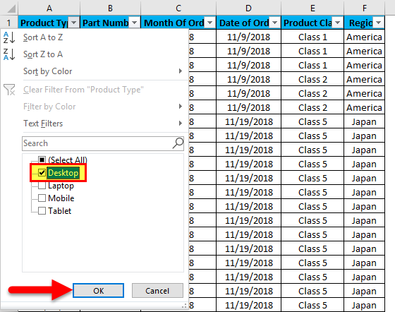
Let us apply the filter and see what changes happen in the data, as seen in the first screenshot, where data is in a randomly scattered format. For that, go to column A, and in the drop-down menu, select only Desktops, as shown in the screenshot below, and click OK.
Once we do it, we will see the data is now filtered with Desktop. And whatever the data is in w.r.t. Desktop, the rest of the columns will also get filtered, as shown in the screenshot below.
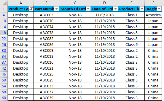
As we can see in the above screenshot, data is now filtered with Desktop, and all the columns are also sorted with data available for Desktop. Also, the line numbers, which are circled in the above screenshot, show the random numbers. This means that the filter we applied was in a random format, so the line numbers were scattered when we applied the filter.
Now, let’s apply the text filter, which is very interesting in filtering the data. For that, go to any of the columns, and click the drop-down button to see the filter options.
Now go to Text Filters.
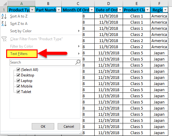
We will find a few more options for filtering the data, as shown in the screenshot below.
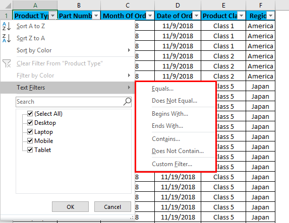
The highlighted portion of Text Filters in the box has Equals, Does Not Equal, Begins With, Ends With, Contains, Does Not Contain, and Custom Filter.
- Equal: With this, we can filter the data with an exact equal word available in the data.
- Does Not Equal: With this, we can filter the data with a word that does not match the available words in the data.
- Begins With: This filters the data, beginning with a specific word, letter, or character.
- Ends With: This filters the data, ending with a specific word, letter, or character.
- Contains: With this, we can filter the data containing any specific word, letter, or character.
- Does Not Contain: With this, we can filter the data which does not contain any specific word, letter, or character.
- Custom Filter: With this, we can apply any combination of the Text mentioned above Filters in data to get data filtered more deeply and specifically to our requirement. Once we click on Custom Filter, we will get a box of Custom AutoFilter, as shown in the below screenshot.
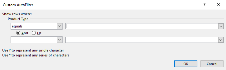
As we can see in the above screenshot of Custom AutoFilter, it has to two filter options at the left sides, which And and Or check-in circles separate. And the other two boxes on the left side are for filling the criteria values. This can be called a smart filter.
There are different ways of applying the Excel column filter.
- Data menu -> Filter
- By pressing Ctrl + Shift + L together.
- By pressing Alt + D + F + F simultaneously.
Pros of Excel Column Filter
- By applying filters, we can sort the data as per our needs.
- By filters, performing the analysis or any work becomes easy.
- Filters sort the data with words, numbers, cell colors, font colors, or with any range. Also, multiple criteria can use.
Cons of Excel Column Filter
- Filters can be applied to all range sizes, but it is not useful if the data size increases to a certain limit. In some cases, if the data goes beyond 50,000 lines, it becomes slow, and sometimes it does not show data available in any column.
Things to Remember
- If you are using the filter and freeze panel together, apply the filter and then use the freeze panel. By doing this, data will be frozen from the middle portion of the sheet.
- It will take a lot more time to apply, and sometimes the file also gets crashes. Avoid or be cautious while using a filter for huge data sets (maybe for 50000 or more).
Recommended Articles
This has been a guide to Filter columns in Excel. Here we discuss how to filter a column in Excel, practical examples, and a downloadable Excel template. You can also go through our other suggested articles –
