Seaborn Correlation Heatmap

Updated March 17, 2023

Introduction to Seaborn Correlation Heatmap

Seaborn correlation heatmap showed a matrix of 2D correlation between dimensions, which was discrete. It will show the dimensions using colored cells to represent monochromic data from the scale. The first dimension value will appear as the table rows, while the second dimension will appear as a table column. The cell color is proportional to the number of measurements matching the dimensional value of the heatmap.

Key Takeaways

• It is an axis-level function used to draw the heatmap into the axis currently active if suppose; we have not provided an ax argument.
• The axis space is taken and used in a colormap plot unless we provide a separate axis.

What is Seaborn Correlation Heatmap?

The dimensional values make it ideal for data analysis since it will make the pattern easy to highlight the difference in the data variation. A regular heatmap is assigned using a colorbar to make the data understandable and readable.

For the analysis of data, a correlation heatmap is very useful. It will explain to us how data elements are interrelated with one another. The correlated value varies from -1 to +1. The correlation will indicate that independent quantities are unrelated to one another. The positive correlation heatmap means the element is working correctly, whereas the negative correlation heatmap will move in a different direction. By using the seaborn package, we can visualize the matrix of correlation. It will simplify analyzing the data source employed in the analytical work.

How to Create Seaborn Correlation Heatmap?

The seaborn is built onto the data visualization library of a matplotlib. To create it, first, we need to install the seaborn library on our system. Also, we need to import the seaborn and matplotlib module into our system.

To create it, we need to follow the below steps as follows:

• First, we need to install the seaborn library in our system.
• After installing the library, we need to import the required libraries. We need to import the numpy, seaborn, and matplotlib libraries.
• We also need to import the file or data set from where we have stored the data or from whom we have fetched the data.
• After retrieving the data, we plot the heatmap using the heatmap method.
• After plotting it, we display the same using the show method.

The below syntax shows the seaborn correlation heatmap as follows. In function, the data parameter is required, except all the parameters of the seaborn correlation heatmap are optional.

Syntax:

Seaborn.heatmap(parameters)

The below example shows how we can create the seaborn correlation heatmap as follows. In the below example, we are reading the csv file by using the read_csv function; we are using the cmap function as Blues as follows.

Code:

import matplotlib.pyplot as plt
import pandas as pd
import seaborn as sb
plot = pd.read_csv("correlation_heatmap.csv")
print(plot.corr())
dataplot = sb.heatmap (plot.corr(), cmap = "Blues", annot = True)
plt.show()

Output:

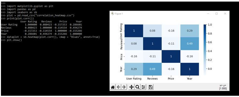
In the above example, we have used the cmap parameter.

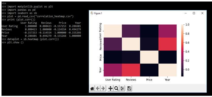
In the below example, we are not using any parameter. We are using only data parameters for creating it.

Code:

import matplotlib.pyplot as plt
import pandas as pd
import seaborn as sb
plot = pd.read_csv("correlation_heatmap.csv")
print (plot.corr())
dataplot = sb.heatmap (plot.corr())
plt.show ()

Output:

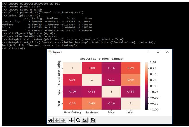
We are using vmin and vmax parameters in the example below to create it.

Code:

import matplotlib.pyplot as plt
import pandas as pd
import seaborn as sb
plot = pd.read_csv("correlation_heatmap.csv")
print (plot.corr())
plt.figure(figsize = (6, 6))
dataplot = sb.heatmap(plot.corr(), vmin = -1, vmax = 1, annot = True)
dataplot.set_title ('Seaborn correlation heatmap', fontdict = {'fontsize':10}, pad = 10);
plt.show()

Output:

Seaborn Correlation of Two Variables

We can define the seaborn correlation ship between dependent and independent variables. In the example below, we create the color map showing the correlation strength between independent variables, including our dependent variable module. The following example will return the correlation of the dependent variable as follows.

Code:

import matplotlib.pyplot as plt
import pandas as pd
import seaborn as sb
plot = pd.read_csv("correlation_heatmap.csv")
print (plot.corr())
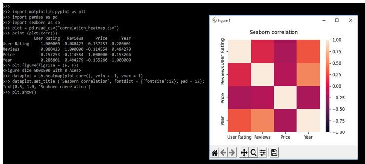
plt.figure(figsize = (5, 5))
dataplot = sb.heatmap(plot.corr(), vmin = -1, vmax = 1)
dataplot.set_title ('Seaborn correlation', fontdict = {'fontsize':12}, pad = 12);
plt.show()

Output:

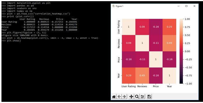
In the below example, we are using the vmin and vmax variables as follows. Also, we are using annot variables as follows.

Code:

import matplotlib.pyplot as plt
import pandas as pd
import seaborn as sns
import numpy as np
plot = pd.read_csv("correlation_heatmap.csv")
print (plot.corr())
plt.figure(figsize = (5, 5))
plot = sb.heatmap(plot.corr(), vmin = -1, vmax = 1, annot = True)
plt.show()

Output:

Examples of Seaborn Correlation Heatmap

Different examples are mentioned below:

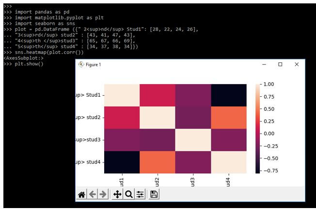
Example #1

In the below example, we are creating our data set as follows.

Code:

import pandas as pd
import matplotlib.pyplot as plt
import seaborn as sns
plot = pd.DataFrame ({ ]
  "3<sup>rd</sup> stud2" : [ ],
  "4<sup>th </sup>stud3" : [ ],
  "5<sup>th</sup> stud4" : [ ]})
sns.heatmap (plot.corr())
plt.show ()

Output:

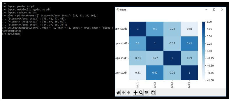
Example #2

In the below example, we are importing the panda’s module.

Code:

import pandas as pd
import matplotlib.pyplot as plt
import seaborn as sns
plot = pd.DataFrame ({ ],
"3<sup>rd</sup> stud2" : [ ],
"4<sup>th </sup>stud3" : [ ],
"5<sup>th</sup> stud4" : [ ]})
sns.heatmap(plot.corr(), vmin = -1, vmax = +1, annot = True, cmap = 'Blues')
plt.show()

Output:

Example #3

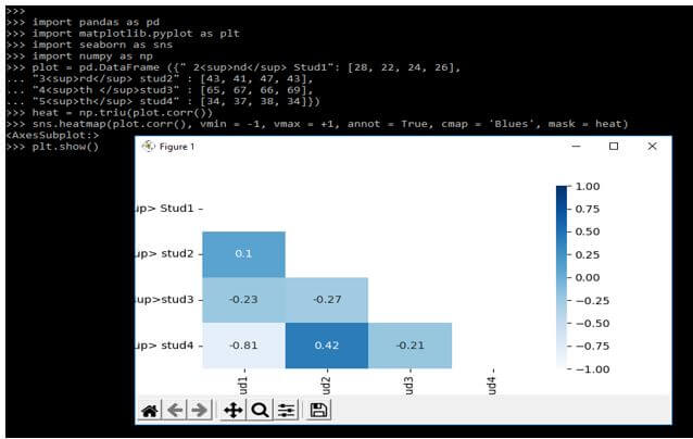
In the below example, we are using the numpy library to define the example.

Code:

import pandas as pd
import matplotlib.pyplot as plt
import seaborn as sns
import numpy as np
plot = pd.DataFrame ({ ],
  "3<sup>rd</sup> stud2" : [ ],
  "4<sup>th </sup>stud3" : [ ],
  "5<sup>th</sup> stud4" : [ ]})
heat = np.triu(plot.corr())
sns.heatmap(plot.corr(), vmin = -1, vmax = +1, annot = True, cmap = 'Blues', mask = heat)
plt.show()

Output:

FAQ

Other FAQs are mentioned below:

Q1. What is the use of the seaborn correlation heatmap in python?

Answer:

It shows the correlation matrix between two dimensions by using colored cells.

Q2. Which libraries do we need to use to plot the seaborn correlation heatmap in python?

Answer:

We need to use the seaborn, numpy, pandas, and matplotlib library while plotting it.

Q3. What is visualizing data correlation in the seaborn correlation heatmap?

Answer:

It is a valuable tool for creating figures that provide insights and trends that quickly identify the potential within a data set.

Conclusion

The correlation will indicate that independent quantities are unrelated to one another. Seaborn correlation heatmap showed a matrix of 2D correlation between dimensions, which was discrete. It will show the dimensions using colored cells to represent monochromic data from the scale.

Recommended Articles

This is a guide to Seaborn Correlation Heatmap. Here we discuss the introduction, creating a seaborn correlation heatmap with examples, and FAQ. You may also have a look at the following articles to learn more –

1. Seaborn barplot
2. Seaborn heatmap
3. Seaborn Scatter Plot
4. Seaborn Histogram