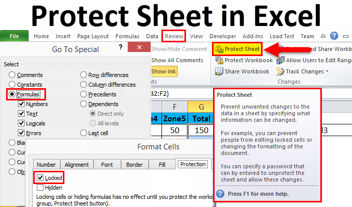
What Does Protect Sheet in Excel Mean?
Protect sheet in Excel is a feature that you can use to lock your Excel worksheet by adding various restrictions and permissions. It allows you to control what others can do with a particular worksheet.
It protects the data present in a workbook or worksheet by adding a password to it. This prevents unauthorized users from changing the protected sheet’s data, such as structure, content, or formatting.
For instance, imagine you add a password to a sales report and share the password only with the sales department. Thus, anyone other than the sales department employee won’t be able to make any changes to the data.
Table of Contents
Why Use Protect Sheet in Excel?
Here are a couple of reasons you might want to use protect sheet in Excel:
- Data Security: You can keep your data safe from accidental changes or unauthorized access.
- Data Integrity: Prevent important formulas or information from being accidentally deleted or modified.
- Collaboration: You can work on a project with others without worrying about them accessing any information that they should not have access to.
How to Protect Sheet in Excel?
You have two options to protect sheet in Excel. You can lock a specific worksheet to stop others from opening it at all, or you can protect specific cells. If you choose the second option, people can open and edit the worksheet, but they won’t be able to make changes to the protected cells.
Follow these steps to protect your sheet in Excel.
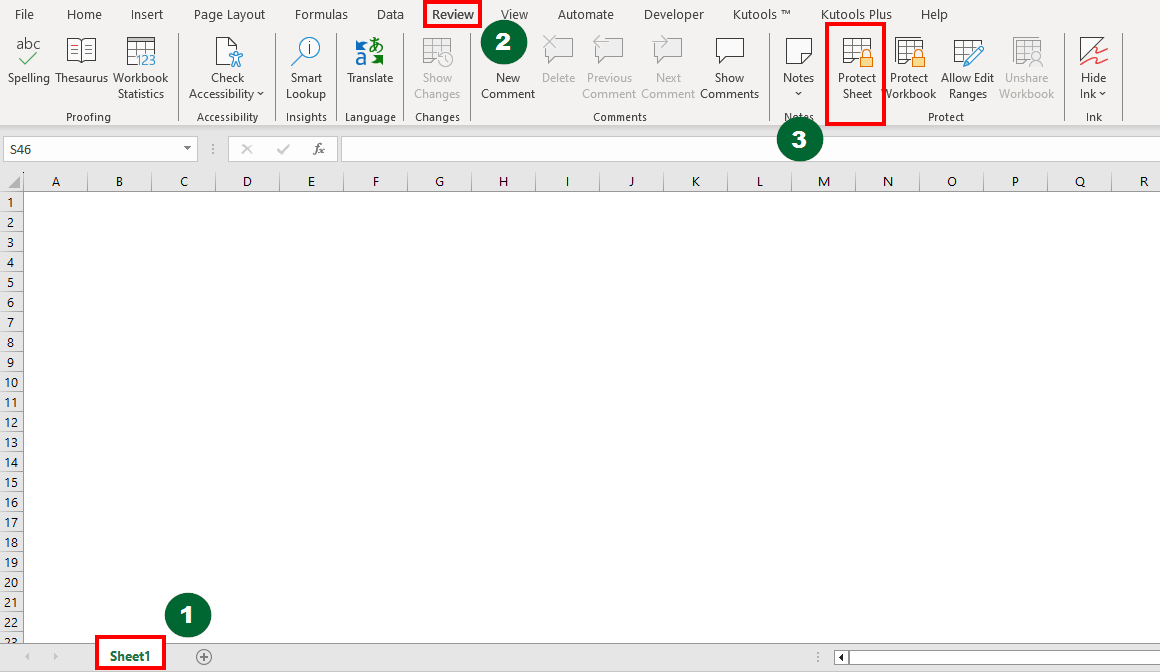
1. Open the Protect Sheet dialog box using the below steps:
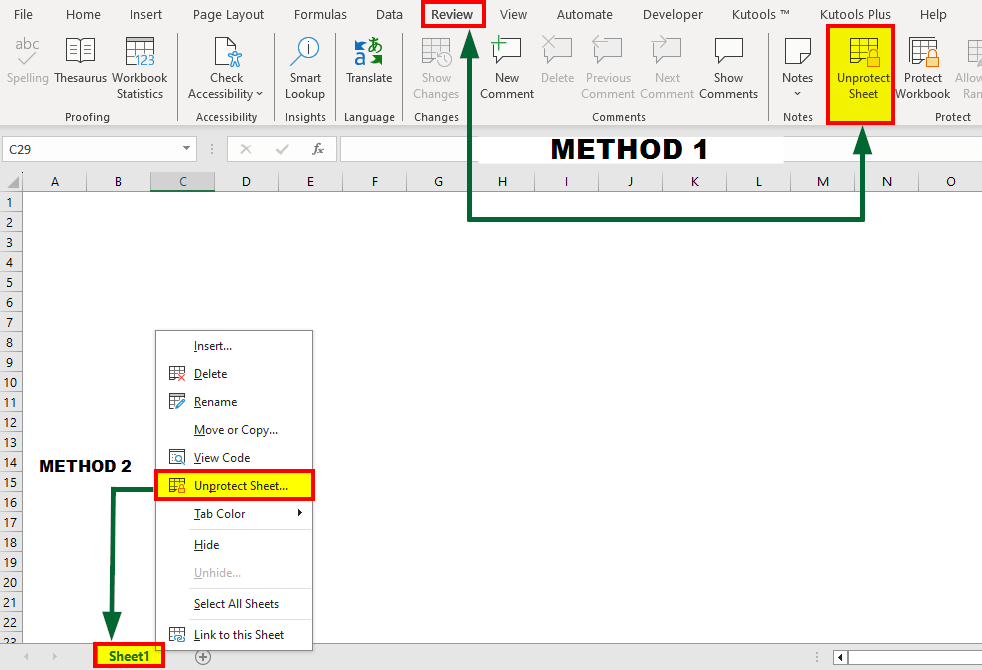
- Step 1: Click on the Sheet1 tab at the bottom of the Excel window.
- Step 2: Open the Review tab from the Excel ribbon.
- Step 3: Under Changes or Protect group, select the Protect Sheet option.
OR
Right-click on Sheet1 and select the Protect Sheet option.
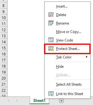
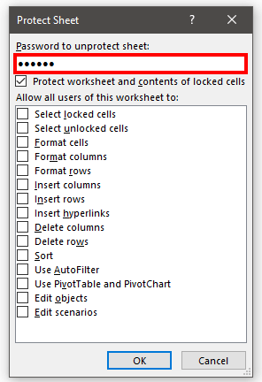
A dialog box will appear.
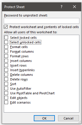
- Set a password as per your choice. Remember this password, as you will need it to unprotect the sheet later.
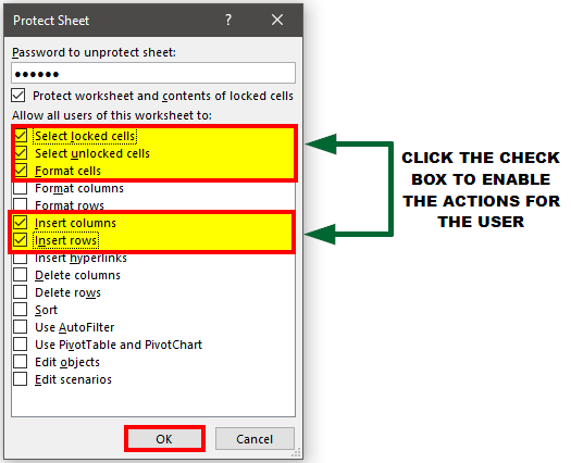
2. If you want the users to be able to do something on the protected sheet, like selecting cells, formatting, etc., just click the checkbox next to that action and Click OK.
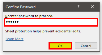
3. Re-enter the password to confirm it, and then click OK.
To cross-check, click on the Review tab OR Right-click on Sheet1 to check. It would show as Unprotect Sheet, meaning that your sheet is already in protection mode.
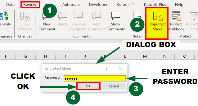
How to Unprotect a Sheet?
To make changes to a protected sheet or to remove protection, follow these steps:
- Go to the Review tab.
- Click on Unprotect Sheet. A Dialog box will appear.
- Enter the password that you set before to unprotect the sheet.
- Click on OK.
How to Lock & Protect Cells in an Excel Worksheet?
It is very simple and easy to protect cells in Excel. Let’s understand the workings of protecting cells in Excel with some examples.
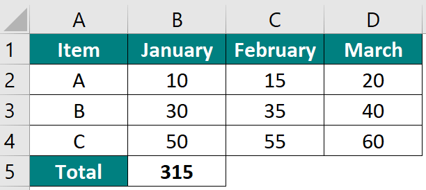
Given:
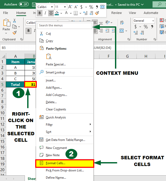
Step 1: Select the cell you want to protect and Right-click. and
Step 2: A context menu will appear. Select the Format Cells option in the context menu.
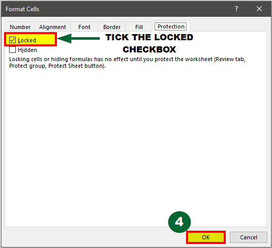
Step 3: In the Format Cells dialog box that appears, go to the Protection tab.
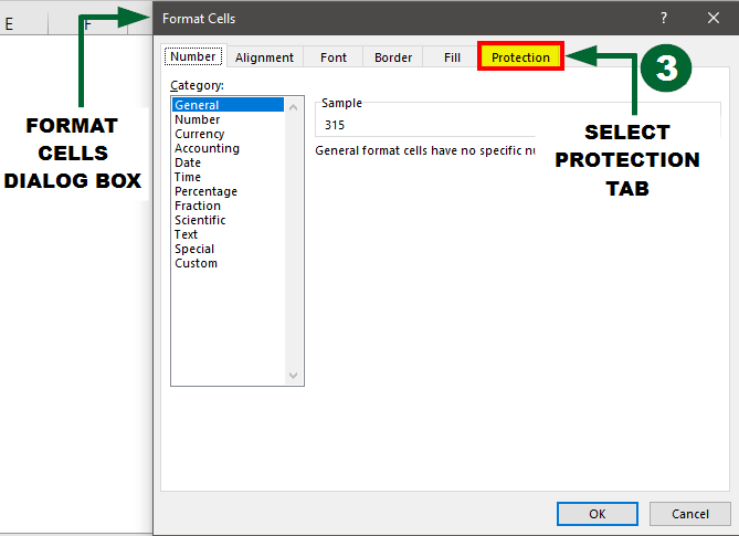
Step 4: You will see that the “Locked” checkbox is ticked by default in Excel. If the checkbox is not selected, then tick the “Locked” checkbox and Click OK.
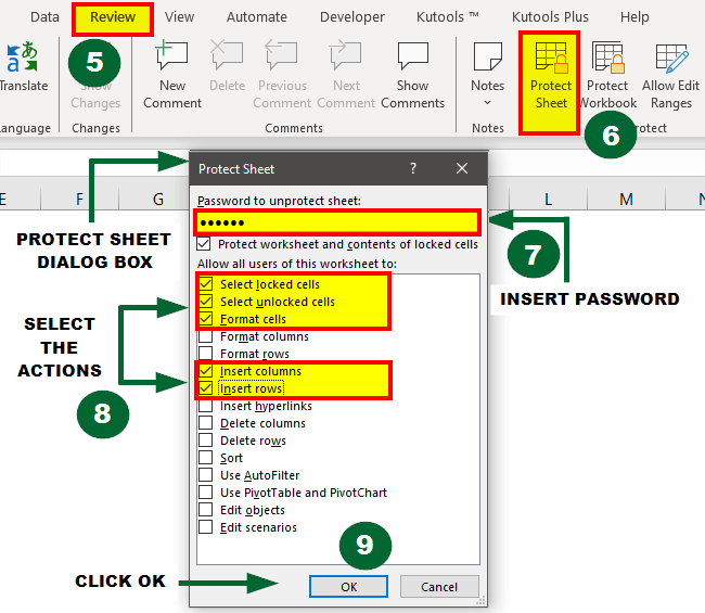
Step 5: Go to the Review tab.
Step 6: Click Protect Sheet.
Step 7: Set a password.
Step 8: Specify the actions users can perform on the protected sheet.
Step 9: Click OK.
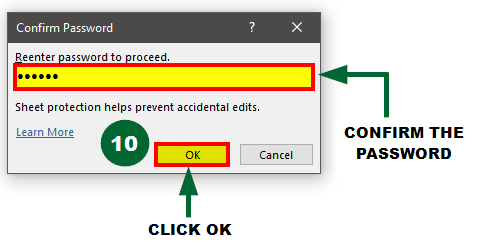
Step 10: Confirm the password to proceed.
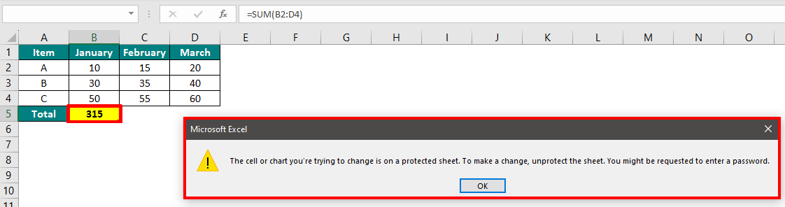
Now, if you try to click on the cell, a message will pop up on your screen (as shown in the below image) stating that the cell is protected. So, to access the particular cell, you will need to enter the password.
How to Hide the Formula within a Cell?
If you want to hide the formula, you can use the below method:
Given:
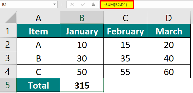
Step 1: Select the cell containing the formula that you want to hide, E.g., B5.
Step 2: Follow these steps:
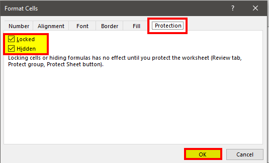
- Right-clicking the cell > Choose Format Cells > Go to the Protection tab.
- Now, instead of only selecting the “Locked” checkbox (as shown in the previous section), you must tick the “Hidden” checkbox as well.
Step 3: Protect the worksheet (see section “How to Protect Sheet in Excel?”).
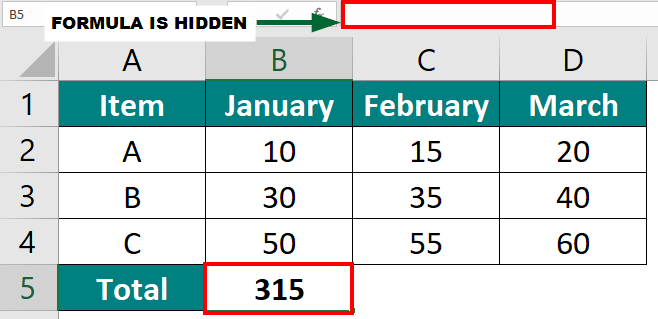
Step 4: Once the cell is protected, the formula will be hidden from view, and users won’t be able to modify it without unprotecting the sheet first.
Result:
Frequently Asked Questions (FAQs)
Q1. Can I lock all the formulas in my worksheet at once?
Answer: Yes, you can lock all the formulas in my worksheet at once. For this, you will first need to select all the formulas and then go ahead and lock the selected cells.
Now, if your Excel sheet has less than 10 formulas, you can easily select them using the mouse or the keyboard shortcut. However, if your sheet has more formulas (Eg, 50), you can use the Go to Special option. It lets you select all formulas in a worksheet at once.
To select all the formulas, follow these steps:
- Go to the Home tab
- Open the Find & Select dropdown menu from the Editing group.
- Click on Go to Special. A dialog box will open.
- Choose the type of data you want Excel to select. For instance, click on the Formulas option box.
- Click the OK button.
You will see that all the formulas that are present in the sheet are selected. Now, you can go ahead and lock the selected cells using the format cells option shown in the section “How to Lock & Protect Cells in an Excel Worksheet?.”
Q2. What is the difference between protect sheet and protect workbook in Excel?
Answer: Protect sheet safeguards individual sheets in Excel by controlling actions within them, such as editing and formatting. On the other hand, protect workbook secures the entire Excel workbook, including all its sheets. It prevents changes to the workbook’s structure, like adding or deleting sheets.
Q3. Can I protect multiple sheets in the same workbook with different passwords?
Answer: Yes, you can protect different sheets in the same workbook with different passwords to provide different levels of access to users.
Q4. What if I want to allow certain users to edit specific parts of a protected sheet?
Answer: You can unlock specific cells or ranges within a protected sheet by unchecking the “Locked” option in the cell formatting and then protecting the sheet. Users will be able to edit only the unlocked cells.
Recommended Articles
This has been a guide to Protect Sheet in Excel. Here, we discuss how to Protect the Sheet in Excel, along with practical examples. You can also go through our other suggested articles-
