List of Basic Formulas and Functions
-
- SUM in Excel
- MAX Formula in Excel
- MIN Formula in Excel
- AVERAGE in Excel
- COUNT in Excel
- COUNTA in Excel
- NOW in Excel
- LEN in Excel
- ABS in Excel
- RAND in Excel
- RANDBETWEEN in Excel
- UPPER in Excel
- LOWER in Excel
- PROPER Function in Excel
What is Excel Formula?
Now, what do you mean by the Excel formula? It sounds like extensive jargon! But don’t worry! Excel formulas make life simple. You can use Excel formulas to calculate numbers with a very dynamic passion. Excel formulas will calculate numbers or values for you so that you don’t have to seat large numbers manually and risk making avoid fakes.
“A formula is an instruction given by the user to carry out some activity within spreadsheet, generally its calculation.”
This is the formal definition of an Excel formula. Our main concern is to learn basic Excel formulas in Excel so let’s look at How to enter a formula in Excel? When you enter an Excel formula, you must be clear about your ideas or what you want to do in Excel. Let’s say you are in one cell and want to enter the formula then; First, you have to start by typing the = (equals) sign, then the remaining formula. Here Excel provides another option for you. Start a formula with a plus (+) or minus (-) sign. Excel will assume that you’re typing a formula, and after pressing enter, you will get your desired Excel formulas result. If you don’t type the equals sign first, then Excel will assume you are typing either a number or a text.
You need to follow some steps to enter a formula into Excel.
- Go to the cell in which you want to enter a formula.
- Either type the equal sign (=) or (+), or (-) sign to tell Excel that you’re entering a formula.
- Type the remaining formula in the cell.
- Lastly, press Enter to confirm the formula.
Take a simple Excel formula with the example; if you want to calculate the sum of two numbers, i.e., 5 & 6 in cell A2, how do you calculate? Let’s follow the above steps:
- Go to the “A2” cell
- Type “=”sign in cell A2
- Then enter the formula; here you have do the sum of 5 & 6, so the formula will be “= 5 + 6”
- Once you complete your formula, then press “Enter”. You will get your desired result, i.e., 11
Many times, instead of getting your desired Excel formulas result, you will encounter an error in Excel. Following are some Excel formula errors faced by many Excel users.
How to Use Basic Formulas in Excel? (Examples)
Excel Basic Formulas is very simple and easy to use. Let’s understand the different Basic Formulas in Excel with some examples.
Formula #1 – SUM Function
I don’t think there is anybody in the university who does not know the summation of numbers. Be it an educated or uneducated, adding numbers skill reached everybody. To make the process easy, Excel has a built-in function called SUM.
We can do the summation in two ways; we need not apply the SUM function; rather, we can apply the calculator technique here.
# Example
Look at the below data. I have a few numbers from cells A2 to A5. I want to do the summation of a number in cell A6.
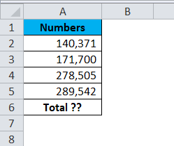
To get the total of the cells A2 to A5. I am going to apply the simple calculator method here. So the result will be:
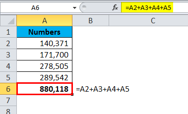
Firstly I selected the first number, cell A2; then I mentioned the addition symbol +; then I selected the second cell and again the + sign, and so on. This is as easy as you like.
The problem with this manual formula is that it will take a lot of time to apply in the case of many cells. I had only 4 cells to add in the above example, but what if there are 100 cells to add? It will be almost impossible to select one by one. That is why we have an inbuilt SUM function to deal with it.
The SUM function requires many parameters, and each is selected independently. If the range of cells is selected, it requires only one argument.
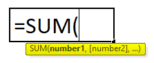
Number 1 is the first parameter. This is enough if the range of cells is selected, or we need to keep mentioning the cells individually.
#Example
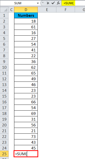
Look at the below example; it has data for 23 cells.
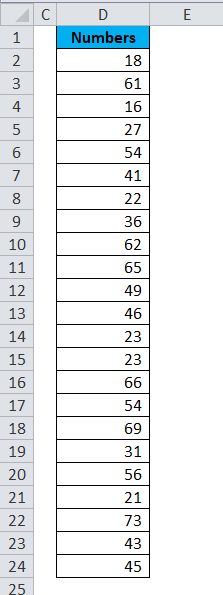
Now open the equal sign in cell D25 and type SUM.
Select the range of cells by holding the shift key.
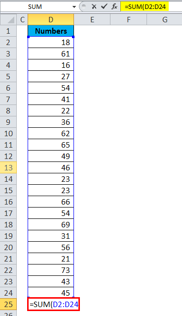
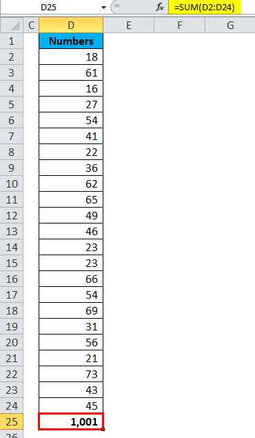
After selecting the range of cells to close the bracket and hitting the enter button, it will summate the numbers from D2 to D24.
Formula #2 – MAX & MIN Function
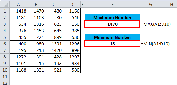
If you are working with numbers, there are instances where you need to find the maximum number and the minimum number in the list. Look at the below data. I have a few numbers from A1 to D10.
#Example
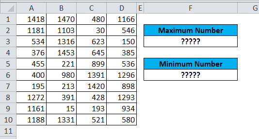
In cell F3, I want to know the maximum number in the list, and in cell F6, I want to know the minimum number. We have the MAX function to find the maximum value; to find the minimum value, we have the MIN function.
Formula #3 – AVERAGE Function
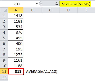
Finding the average of the list is easy in Excel. Finding the average value can be done by using an AVERAGE function. Look at the below data. I have numbers from A1 to A10.
#Example
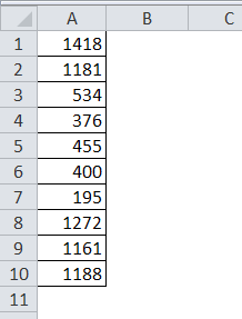
I am applying the AVERAGE function in the A11 cell. So the result will be:
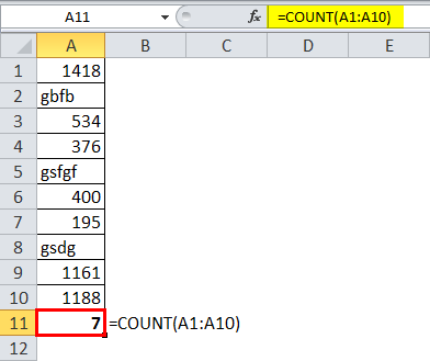
Formula #4 – COUNT Function
The COUNT function will count the values in the supplied range. It will ignore text values in the range and count only numerical values.
#Example
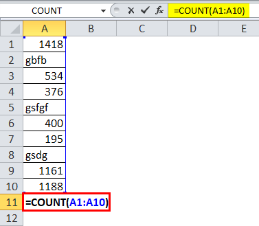
So the result will be:
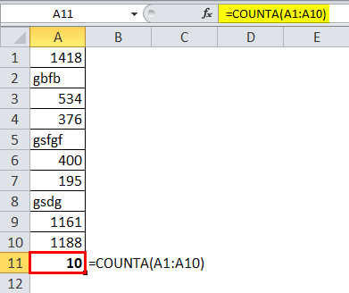
Formula #5 – COUNTA Function
COUNTA function counts all the things in the supplied range.
#Example
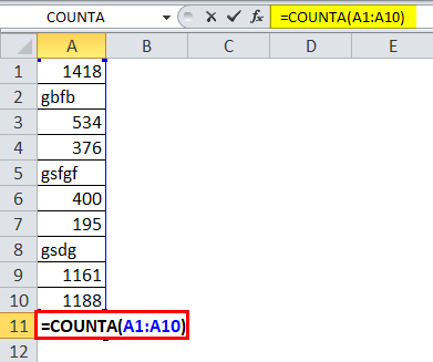
So the result will be:
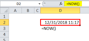
Formula #6 – NOW Function
If you want to insert the current date and time, you can use the NOW function to do the task.
#Example
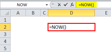
So the result will be:
Formula #7 – LEN Function
You can use the LEN function to know how many characters are in a cell.
#Example
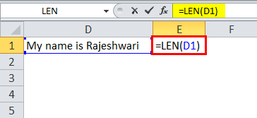
LEN function returns the length of the cell.
In the above image, I have applied the LEN function in cell E1 to find how many characters there are in cell D1. LEN function returns 21 as a result.
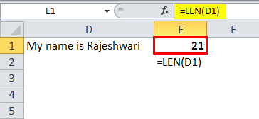
That means in cell D1 total of 21 characters are there, including space.
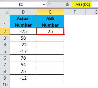
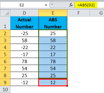
Formula #8 – ABS Function
You can use the ABS function to convert all the negative numbers to positive ones. ABS means absolute.
#Example
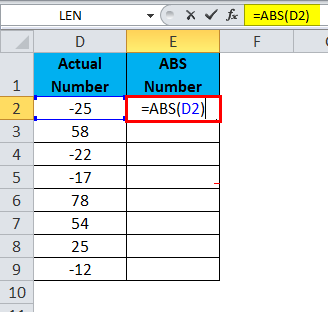
So the result will be:
So the final output will occur by dragging cell E2.
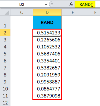
Formula #9 – RAND Function
RAND means random. It is a volatile function. You can use the RAND function to insert random numbers from 0 to less than 1.
#Example
Formula #10 – RANDBETWEEN Function
RAND function inserts the numbers from 0 to less than 1, but RANDBETWEEN inserts numbers based on the numbers we supply. We need to mention the bottom and top values to tell the function to insert random numbers between these two.
#Example
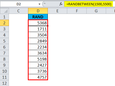
Look at the above image. I have mentioned the bottom value as 1500 and the top value as 5500. Formula inserted numbers between these two numbers.
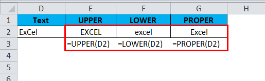
Formula #11 – UPPER, LOWER & PROPER Function
When dealing with the text values, you care about their appearances. If we want to convert the text to UPPERCASE, we can use an UPPER function; we want to convert the text to LOWERCASE, we can use the LOWER function; and if we want to make the text proper appearance, we can use the PROPER function.
#Example
Errors in Excel formulas
How many times have you encountered Excel errors? It’s a frustrating experience when Excel gives an error. Two kinds of Excel formulas error occur in Excel first #VALUE And #NAME. This will happen if the formula you’ve typed is invalid.
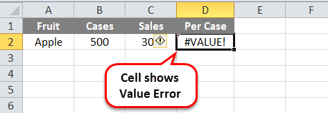
#VALUE Error
This means that you entered a valued formula, but Excel could not calculate a valid result from your formula.
Look at the following picture carefully; two columns consist of the Department and the number of students. Now #VALUE error occurs when you try to calculate Excel formulas to add cells containing the non-numerical value. If you are trying to Add values Cell A2 and B2, then Excel gives you the #VALUE error because Cell A2 contains the non-numerical value.
Reasons for #VALUE Error
- Adding cells that contain a non-numerical value
- Error with formula
- Non-numerical value
This Excel formula error is commonly encountered when the formula isn’t formatted correctly or contains other errors, as seen in the example below.
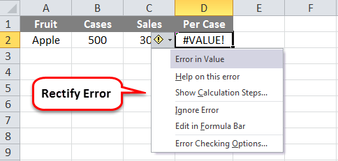
How to Correct #VALUE Error?
Instead of using arithmetic operators, use a function, such as SUM, PRODUCT, or QUOTIENT, to perform an arithmetic operation. Ensure that adding cell does not contain a non-numerical value. The following picture shows how to correct the #VALUE error. In the above example, we have seen why a #VALUE error occurs. Now we are trying to Add cells, including numerical values only. In short, avoid addition, subtraction, division, or multiplication of non-numerical values with numerical values.
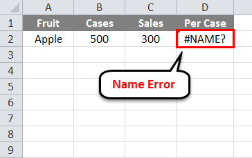
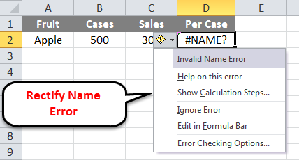
#NAME Error
#NAME error occurs when Excel doesn’t recognize text in a formula. Look at the following picture. What do we do if we want to calculate Excel formulas for the sum of several students? We insert the SUM formula, then select range and press enter. But if you enter formula SUM and select range, then press enter. Excel gives an #NAME error. Because you enter the wrong formula.
How to Correct #NAME Error?
- Ensure the formula is correctly entered.
- Make sure quotation marks are added and balanced from left and right.
- Replacing a colon (:) in a range reference. For e.g. SUM(A1A10) should be COUNT(A1: A10)
Some Basic Arithmetic Excel Formulas
Arithmetic formulas are by far the most common type of formula. It generally includes mathematical operators like Addition, Subtraction, Multiplication, Division, etc., to perform calculations. Look at the following table.
The Arithmetic Operators
| Operator | Name | Example | Result |
|---|---|---|---|
| + | Addition | =5+5 | 10 |
| – | Subtraction | =10-5 | 5 |
| – | Negation | =-10 | -10 |
| * | Multiplication | =10*5 | 50 |
| / | Division | =10/5 | 2 |
| % | Percentage | =10% | 0.1 |
| ^ | Exponentiation | =10^5 | 100000 |
Top 10 Basic Excel Formulas That You Should Know
Don’t waste any more hours in Microsoft Excel doing things manually. Excel formulas decrease your time in Excel and increase the accuracy of your data and reports.
| Name of Formulas | Formula | Description |
|---|---|---|
| SUM | =SUM ( Number1, Number2, … ) | Add all numbers within the range resulted in the sum of all numbers |
| AVERAGE | =AVERAGE(number1, [number2],…) | Calculate average numbers in a range |
| MAX | =MAX( Number1, Number2, … ) | Calculate or find the largest number in a specific range |
| MIN | =MIN( Number1, Number2, … ) | Calculate or find the smallest number in a specific range |
| TODAY | =TODAY() | Returns the current date |
| UPPER | =UPPER(text) | Converts text to uppercase. |
| LOWER | =LOWER(text) | Converts text into lowercase. |
| Countif | =COUNTIF(range, criteria) | This function counts the number of cells within a range that meet a single criterion that you specify. |
| counta | = COUNTA(value1, [value2], …) | This function counts the number of cells that are not empty in a range. |
| ABS | = ABS(number) | The ABS function returns a value of the same type passed to it, specifying the absolute value of a number. |
Recommended Free Formulas Training
If you search on Google for free Excel courses, you may get a long list of free Excel training courses. However, you might get confused by referring to so many Excel resources. I suggest you go for EduCBA’s free online training on Excel. Online courses are much better than expensive classroom training courses because they provide time flexibility and cost-effectiveness. The Excel formulas learning materials are freely available on the EduCBA website, and the videos included in the course are short and very easy to understand, planned especially for beginners. Also, for your convenience, the spreadsheets explained in the videos are available for download. This way, you can immediately practice what you have just seen and learned.
Free Demo Excel
Recommended Articles
Here are some articles that will help you to get more detail about the Excel Formulas Useful For Any Professionals, so go through the link.
