Updated June 12, 2023
Conditional Formatting for Dates in Excel (Table of Contents)
Conditional Formatting for Dates in Excel
Conditional formatting for dates in Excel means it formats the particular data per your criteria. Here we will discuss formatting dates to highlight/format the dates we want in a particular format. The selected dates, i.e., the dates before today, dates of Sundays, weekends, and many more.
Here in Excel, we can select the rules already there or make our own rule and make our desired condition to find/format the desired data. First, let’s see the path to get into conditional formatting.
Step: 1
- First of all, we need to select the data which we need to be formatted.
Step: 2
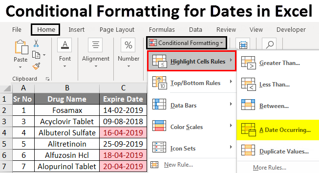
- Click Home from the Menu Bar and click the Conditional Formatting as per the below screenshot.
- The above screenshot shows the options available for conditional formatting by clicking the conditional formatting from the toolbar.
- Now the options available for us are many, but here we have to use them to format the dates.
Step: 3
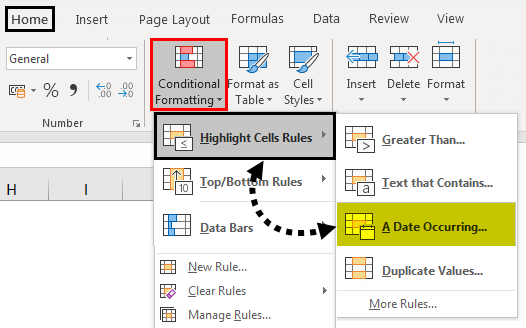
- From the screenshot, we can see a sub-option available of A Date Occurring under the category of highlighting cell rules; clicking the box below will open to show you some options to highlight the particular dates.
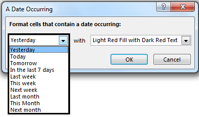
- Here we have an option to highlight the Date from yesterday to next month, and we also have the built-in option of how we want these dates to be highlighted. Like the color of the text and the colored cell, there are some fixed options. Kindly see the following image for the reference of the options available.
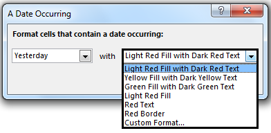
- As you can see, there is also an option of custom format, what more, we need. So we can format our required date in our required color and much more, then click OK, and we shall have our formatted dates.
How to Use Conditional Formatting for Dates in Excel?
As we have seen in the above examples, the conditional formatting for dates can be used in situations like Found duplicate dates or highlighting the required dates of the week by making formula, and we can highlight the dates which are on Monday, Sunday or any other day of the week.
Using built-in options, we can highlight the dates of Yesterday, Today Next Month, or if the built-in option is not usable for us, we can make our own rules. We can format the data as we want using formulas like a weekday, today, date, and Now.
Example #1 – Highlight the Dates of Next Week
For this example, we will see the basic example highlighting last week’s dates.
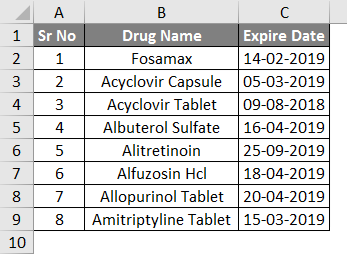
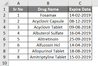
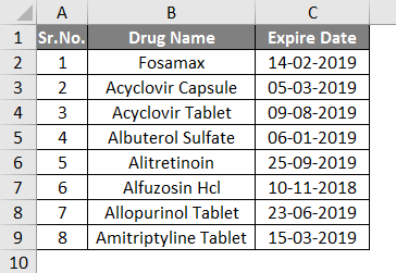
Suppose we have data on the drug with its expiry dates as follows.
- Now we will select all dates, go to the conditional formatting tool from the Home menu, and select the A Date Occurring.
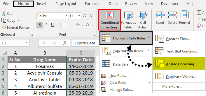
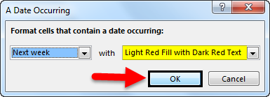
- As we want the next week’s dates, we have selected the “Next week” option, and for formatting, we have selected the “Light Red Fill with Dark Red text.”
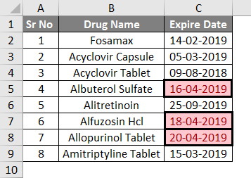
- As we can see from the screenshot below, two drugs have an expiry date of next week, highlighted with Light Red and filled with Dark Red text as required.
Similarly, we can do the same to highlight the dates of Yesterday to Next Month from built-in options.
Example #2 – Highlight Dates of Weekends
For this example, we must explore making new rules, as no built-in option exists to highlight the weekend dates. Suppose we have data on the drug with its expiry dates as follows.
- As no built-in option is available to highlight the weekends, we need to make a rule which identifies the weekend from the given dates and then format and highlight the weekends.
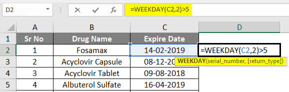
- So first of all, here we need the formula to identify the dates weekends from the given dates; we can use the formula =weekday.
- The logic we can use with this formula is =weekday(serial_number, [return_type])
- Here we have serial number C2 to C9, return value will be in column # 2,
- The logic for this formula is we highlight the date for which the weekday is greater than 5.
- So the formula is =weekday(C2, 2)>5
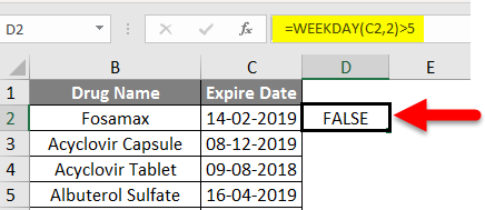
- The output is given below.
- Now repeat the steps, select the date cells C2 to C9, and now click on Conditional Formatting.
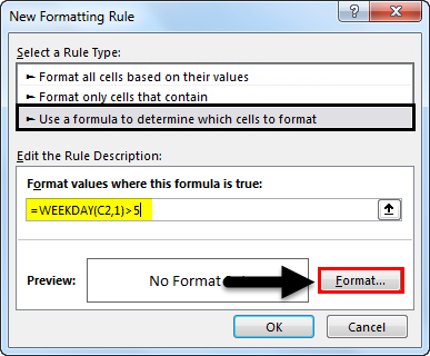
- Click on New Rule.
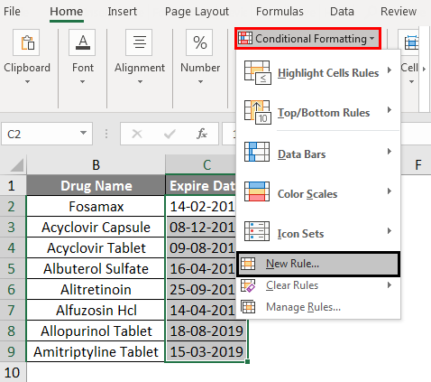
- Select the option. Use a formula to determine which cell to format.
- Now enter our formula =weekday(C2, 2)>5.
- Then select the format by clicking the format button.
- A box, “Format Cells,” will open, and we can fill any color we want.
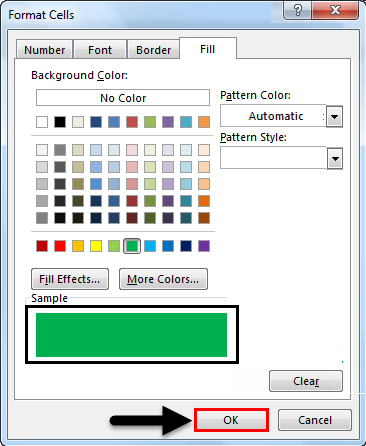
- Here we have taken Green color; by clicking ok, we will have our weekend dates available in Green filling as per the below image.
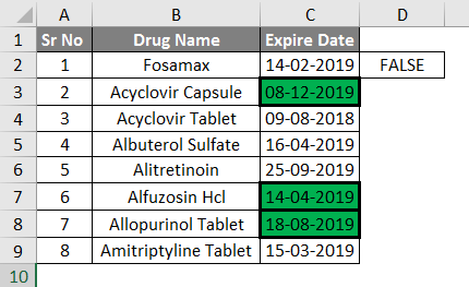
- As per the results, three expiry dates are at weekends.
Example #3 – Highlight the Dates Past Today
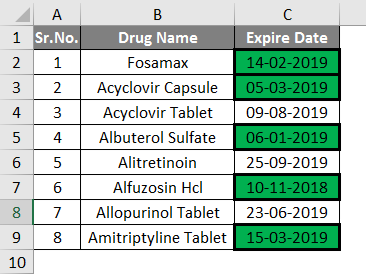
Suppose we have the data for this example as per the image below.
- We want to highlight the dates past today (09/04/2019), so which dates before 09th April 2019 will be highlighted.
- So for this operation, we do not have any built-in option available.
- Here we can do this operation by using the =NOW() function
The steps will be as follows:
- Select the Expiry Dates from the column.
- Click on the Conditional Formatting and click on New Rule.
- A box will open, selecting the Rule type Format only Cells that contain.
- In the rule description, select Cell Value in the first box and Less than in the second box, and type =NOW() function in the third box.
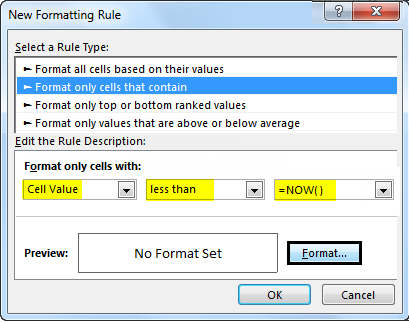
- Now click on format and select the color format according to your choice, and we’re done.
- Here, for example, we have used a Green color.
- And click on Ok.
As per the below image, we can see that the dates which are in the past tense are now formatted in Green color.
- You might think that it is much easier to do this manually, but when we have larger data, it will be very useful, and also, we can use it on a very large scale.
Things to Remember about Conditional Formatting for Dates in Excel
- To apply this conditional formatting, there are things to remember.
- Before applying the formatting, we have to select the columns for which the formatting needs to be applied.
- While creating a new rule, the formula should be applied before applying the formatting to verify the logic.
Recommended Articles
This is a guide to Conditional Formatting for Dates in Excel. Here we discussed using conditional formatting for Dates in Excel and practical examples, and a downloadable Excel template. You can also go through our other suggested articles to learn more –
