Updated June 2, 2023
Conditional Formatting in Excel Pivot Table (Table of Contents)
Conditional Formatting in the Pivot Table
To apply Conditional Formatting in any pivot table, first, select the pivot, and then from the Home menu tab, select any of the conditional formatting options. If you want to format the data with Above Average values under Top/Bottom Rules, choose the option. After that, from the corner of the cell, we will have the Formatting Option icon; from there, select the formatting rule for All the cells there in the pivot showing the value as per the defined or selected condition.
How to Apply Conditional Formatting in Excel Pivot Table?
If you want to highlight a particular cell value in the report, use conditional formatting in the excel pivot table. Let’s take an example to understand this process.
Example #1
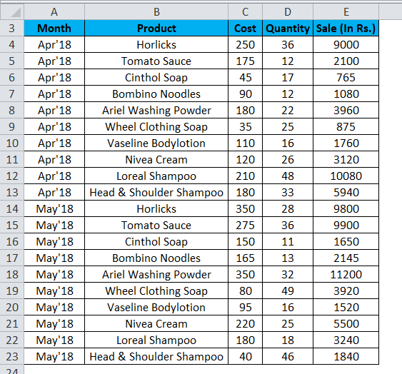
We have given below data of a Retail Store (2 months data).
Follow the below steps to create a Pivot Table:
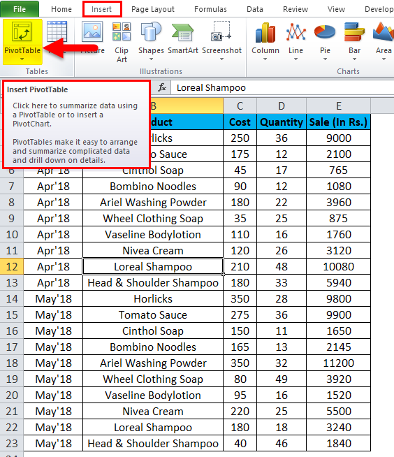
- Click on any cell in the data. Go to the INSERT tab.
- Click on the Pivot Table under the Tables section and create a pivot table. Refer to the below screenshot.
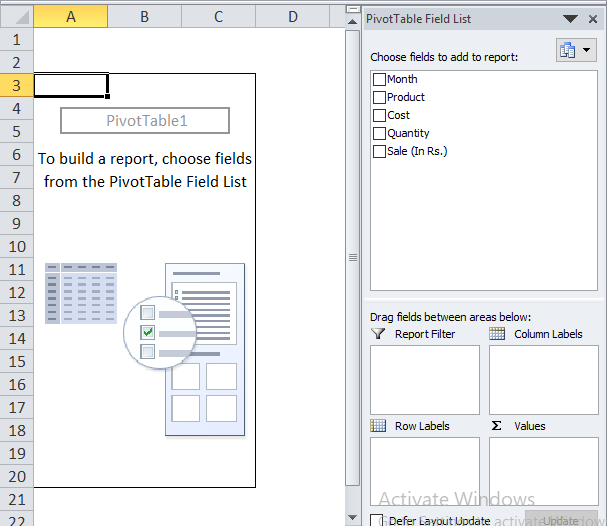
- A dialog box appears. Click OK.
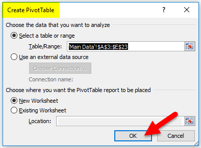
- We get the below result.
- Drag Product field to Rows section, Sales to value section, whereas the Month field to Column section.
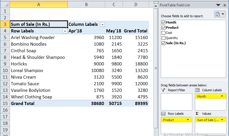
Now we have the Pivot report for month-wise sale. We want to highlight the products whose sale is less than 1500.
For applying conditional formatting in this pivot table, follow the below steps:
- Select the cells range for which you want to apply conditional formatting in excel. We have selected the range B5:C14 here.
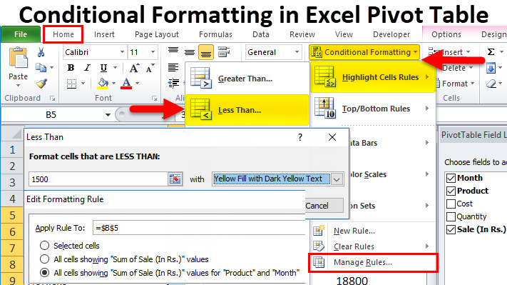
- Go to the HOME tab > Click on Conditional Formatting option under Styles > Click on Highlight Cells Rules option > Click on Less Than option.
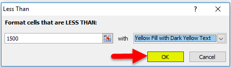
- It will open a Less Than dialog box.
- Enter 1500 under the Format Cells field and choose a color as “Yellow Fill with Dark Yellow Text”. Refer to the below screenshot.
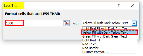
- And then click on OK.
- The Pivot Report will look like this.
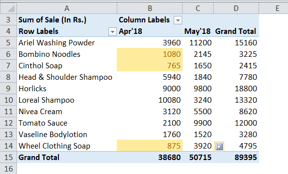
This will highlight all the Cell values which are less than Rs 1500.
But there is a loophole with the condition formatting here. Whenever we make any changes in the Excel Pivot data, then conditional formatting will not be applied to the correct cells, and it might not include the whole new data.
The reason being is when we select a particular cell range for applying conditional formatting in excel. Here we have selected the fixed cell range B5:C14; hence, it would not be applied to the new range when we update the Pivot table.
A solution to overcome the problem:
For overcoming this problem, follow the below steps after applying conditional formatting in the Excel pivot table:
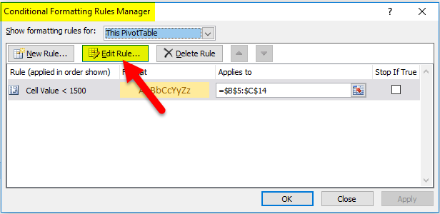
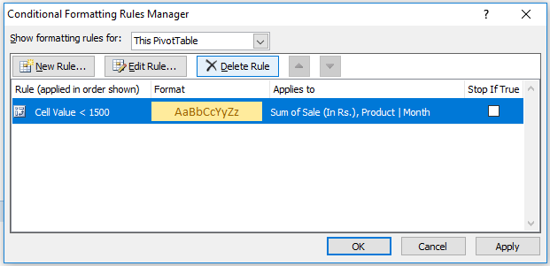
- Click on any cell in the pivot table > Go to the HOME tab > Click on Conditional Formatting option under Styles option > Click on Manage Rules option.

- It will open a Rules Manager dialog box. Click on the Edit Rule tab, as shown in the below screenshot.
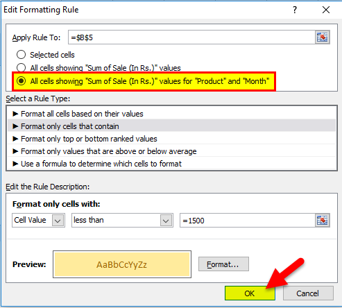
- It will open the Editing Rule formatting window. Refer to the below screenshot.
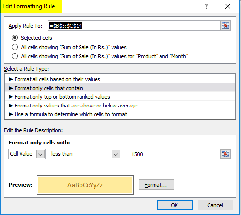
As we can see in the above screenshot, Under Apply Rule To section, there are three options available:
- Selected Cells: This option is not applicable when you make any changes in the Pivot data, like add or delete the data.
- All cells showing “Sum of Sale” values: This option might include extra fields like Grand Totals etc. ,fields which we might not want to include in our reports.
- All cells showing “Sum of Sale” values for “Product” and “Month”: This option restricts with the data and does formatting with cells where our required cells appear. It excludes the extra cells like Grand Totals etc. This option is the best option for formatting.
- Click on the 3rd option All Cells showing “Sum of Sale” values for “product” and “Month” as shown in the below screenshot ,and then click on OK.
- The below screen will appear.
- Click on Apply and then click OK.
It will apply the formatting in all the cells with the updated record in the dataset.
Things to Remember
- If you want to apply a new condition or change the formatting color, you can change these options under the Edit Rule Formatting window.
- This is the best option to present the data to the management and target the specific data which you want to highlight in your reports.
Recommended Articles
This has been a guide to Conditional Formatting in the Pivot Table. Here we discuss how to apply conditional formatting in an excel pivot table along with practical examples and a downloadable excel template. You can also go through our other suggested articles –
