Updated May 29, 2023
Pivot Table Filter in Excel (Table of Contents)
Introduction to Pivot Table Filter
A Pivot Table filter is something that we get when we create a pivot table by default. First, create a table using a Pivot Table; the first field, either a Row or Column, will have one filter. Click on the drop-down arrow or press the ALT + Down navigation key to enter the filter list. In that drop-down list, we have traditional filter options. In another way, we can filter the data by clicking right on those fields.
Let’s look at the multiple ways of using the filter in PIVOT.
How to Filter a Pivot Table in Excel?
Let us see some examples and their explanation of the Filter Pivot Table in Excel.
Example #1 – Creating Inbuilt Filter in PIVOT Table
Step 1: Let’s have the data in one of the worksheets.
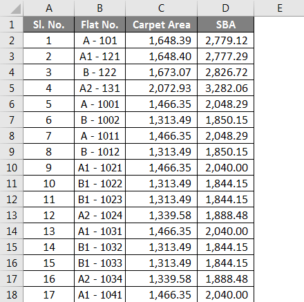
The above data consists of 4 columns with Sl.No, Flat No’s, Carpet Area & SBA.
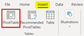
Step 2: Go to the Insert tab and select the Pivot table, as shown below.
The “Create Pivot Table” window pops out when you click the pivot table.
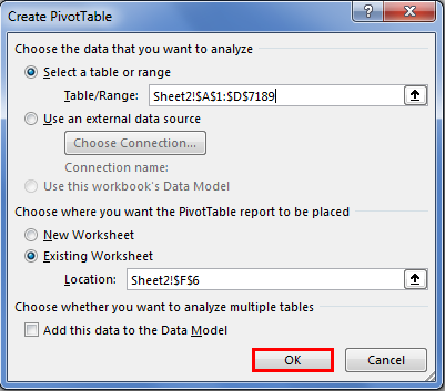
We have an option of selecting a table or a range to create a pivot table, or we also can use an external data source as well. We can also place the Pivot table report in the same or a new worksheet, and we can see it as shown in the above image.
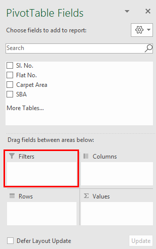
Step 3: Pivot table Field will be available on the right end of the sheet as below. We can observe the Filter field, where we can drag the fields into filters to create a filter in the Pivot table.
Let’s drag the Flat no’s field into Filters, and we can see the filter for Flat no’s would have been created.
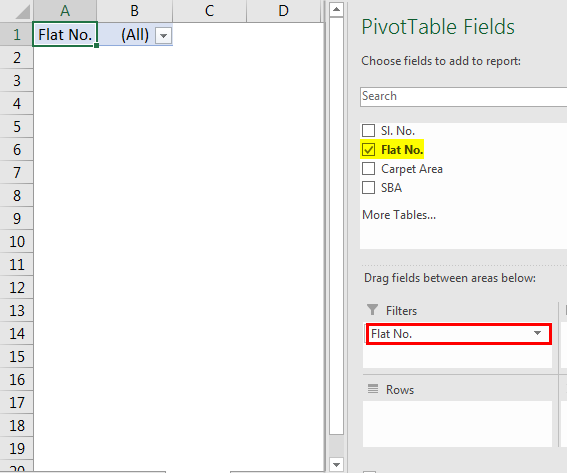
We can filter the Flat no’s as per our requirement, which is the normal way of creating a filter in the Pivot table.
Example #2 – Creating a Filter to the Value Areas
Generally, when we take data into value areas, any filter won’t be created for those fields. We can see it below.
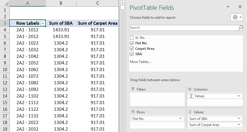
We can observe no filter option for value areas, i.e., the Sum of SBA & Carpet Area. But we can create it and which helps us for various decision-making purposes. Firstly, we must select any cell next to the table and click on the filter in the data tab. We can see the filter gets in the value areas.
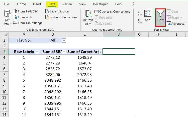
As we get the filters, we can perform different operations from value areas, like sorting them from largest to smallest, to know top sales/area/anything. Similarly, we can sort from smallest to largest, sorting by color, and even perform number filters like <=,<,>=,>, and many more. This plays a major role in decision-making in any organization.
Example #3 – Displaying List of Multiple Items in a Pivot Table Filter
In the above example, we learned to create a filter in Pivot. Now let’s look at how we display the list differently. 3 most important ways of displaying a list of multiple items in a pivot table filter are:-
- Using Slicers
- Creating a list of cells with filter criteria
- List of Comma Separated Values
1. Using Slicer
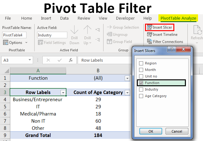
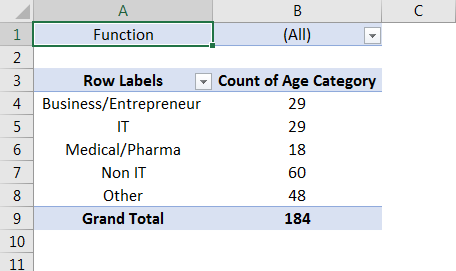
Let’s have a simple pivot table with columns like Region, Month, Unit no, Function, Industry, and Age Category.
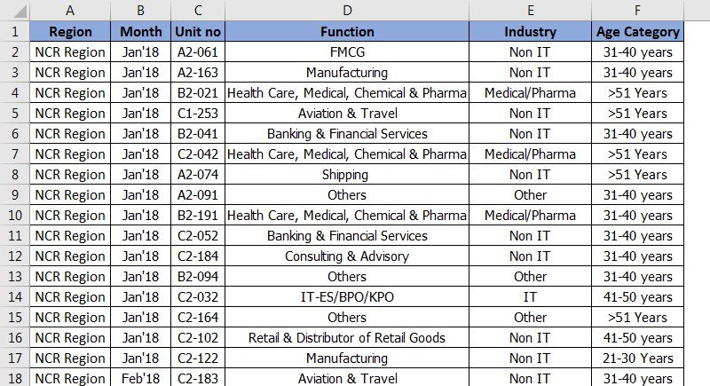
From this example, we will consider Function in our filter and check how it can be listed using slicers and varies as per our selection.
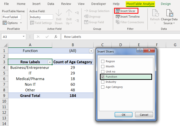
It is simple as we just select any cell inside the pivot table, we’ll go to analyze tab on the ribbon and choose insert slicer, and then we’re going to insert the slicer in our filter area, so in this case, the “Function” filed in our filter area and then hit Ok and that’s going to add a slicer to the sheet.
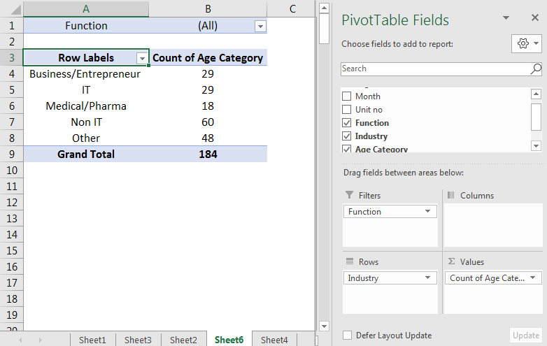
We can see items highlighted in the slicer are highlighted in our filter criteria in the filter drop-down menu. Now, this is a pretty simple solution that does display the filter criteria. We can easily filter out multiple items and see the result varying in value areas. From the below example, it is clear that we had selected the functions that are visible in the slicer and can find out the count of age category for different industries (which are row labels that we had dragged into the row label field), which are associated with those function that is in the slicer. We can change the function according to our requirement and observe the results vary as per the items selected.
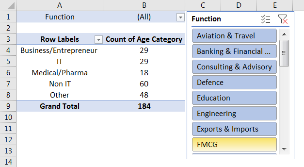
However, if you have a lot of items in your list here and it’s long, then those items might not be displayed properly, and you might have to do a lot of scrolling to see which items are selected so that it leads us to the nest solution of listing out the filter criteria in cells.
So, “Create List of cells with Filter Criteria” comes to our rescue.
2. Create a List of Cells with Filter Criteria:
We’re going to use a connected pivot table, and we’re going to use the above slicer here to connect two pivot tables together. Now let us create a duplicate copy of the existing pivot table and paste it into a blank cell of a new sheet.
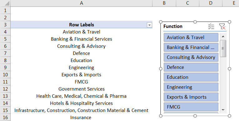
So now we have a duplicate copy of our pivot table, and we will modify it slightly to show that Functions field in the rows area. To do this, we have to select any cell inside of our pivot table here and go over to the pivot table field list and going. To remove Industry from the rows, remove Count of Age Category from the values area. We are going to take the Function in our filters as rows area, and now we can see that we have a list of our filter criteria. If we look over here in our filter drop-down menu, we have the list of items in slicers and function filter.
Now we have a list of our filter criteria, which works because the slicer connects both pivots. If we right-click anywhere on the slicer & report connections – pivot table connections, it will open up a menu showing us that both pivot tables are connected as checkboxes are checked.
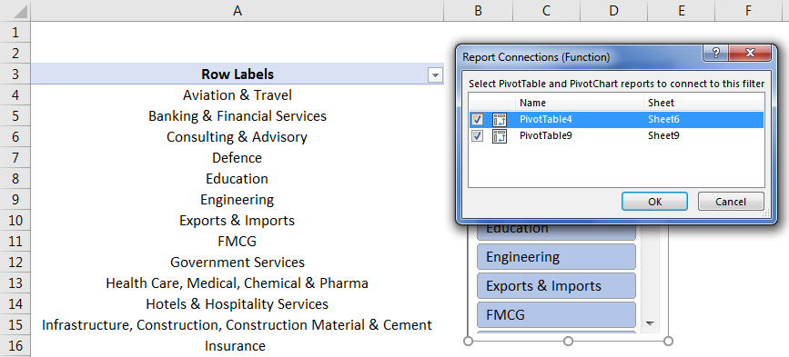
This means whenever one change is made in 1st pivot, it automatically gets reflected in the other. Tables can be moved anywhere, they can be used in any financial model, and row labels can also be changed.
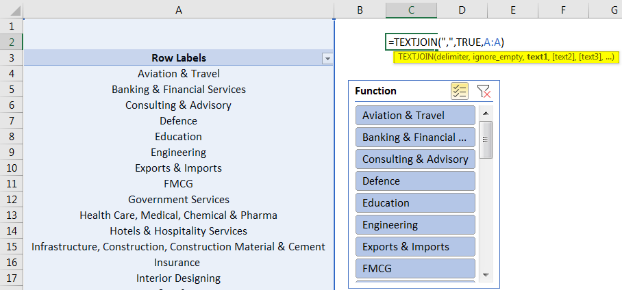
3. List of Comma Separated Values:
So the third way to display our filter criteria is in a single cell with a list of comma-separated values, and we can do that with the TEXTJOIN function. We still need the tables we used earlier and use the formula to create this string of values and separate them with commas.
This is a new formula or function introduced in Excel 2016 & it’s called TEXTJOIN (If you do not have Excel 2016, you can use concatenate function as well); Text joining makes this process much easier.
TEXTJOIN gives us three different arguments.
Delimiter – which can be a comma or space.
Ignore Empty – true or false to ignore empty cells or not.
Text – add or specify a range of cells that contain the values we want to concatenate.
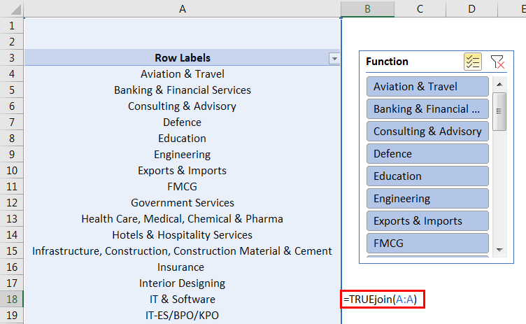
Let us type text join- (delimiter- which would be “,” in this case, TRUE (as we should ignore empty cells), A: A (as the list of selected items from the filter will be available in this column) to join any value & also ignore any empty value in Pivot Table Filter)
Now we see getting a list of all our filter criteria joined by a string. So it’s a comma-separated list of values, and if we didn’t want to show these filter criteria in the formula, we could hide the cell.
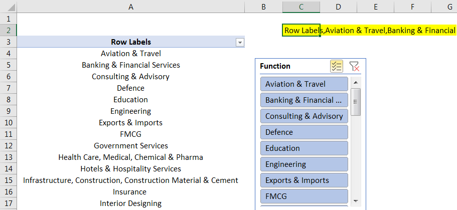
Just select the cell and go up to analyze options tab; click on field headers & which will hide the cell.
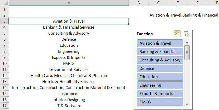
So now we have the list of values in their filter criteria. Now, if we change the pivot filter, it reflects in all the methods. We can use any one of there. But eventually, for a comma-separated solution slicer & the list is required. They can be hidden if you don’t want to display the tables.
Things to Remember
- Filtering is not additive because when we select one criterion and if we want to filter again with another criterion, the first one will be discarded.
- We got a special feature in the filter, i.e., “Search Box”, which allows us to manually deselect some of the results we don’t want. For Ex: If we have a huge list and there are blanks too, then to select blank, we can easily get selected by searching for blank in the search box rather than scrolling down till the end.
- We are not supposed to exclude certain results with the condition in the filter, but we can do this by using a “label filter”. For Ex: If we want to select any product with a certain currency like the rupee or dollar, we can use a label filter – ‘does not contain’ and give the condition.
Recommended Articles
This is a guide to Pivot Table Filter in Excel. Here we discuss How to Create a Pivot Table Filter in Excel, examples, and an Excel template. You can also go through our other suggested articles to learn more –
