Updated June 2, 2023
Numbering in Excel
There are various ways of numbering in Excel: Fill Handle, Fill Series, and Row Function. By Fill Handle, we can drag already written 2-3 numbers in sequence until the limit we want. By Fill Series, which is available in the Home menu tab, select the Series option, and select the lowest and highest numbers. And if we select the Row function for numbering, we can also create a number in the sequence.
How to Add Serial Number in Excel?
To add a serial number in Excel is very simple and easy. Let’s understand the working of adding a serial number in Excel by some methods with its example.
Example #1 – Fill Handle Method
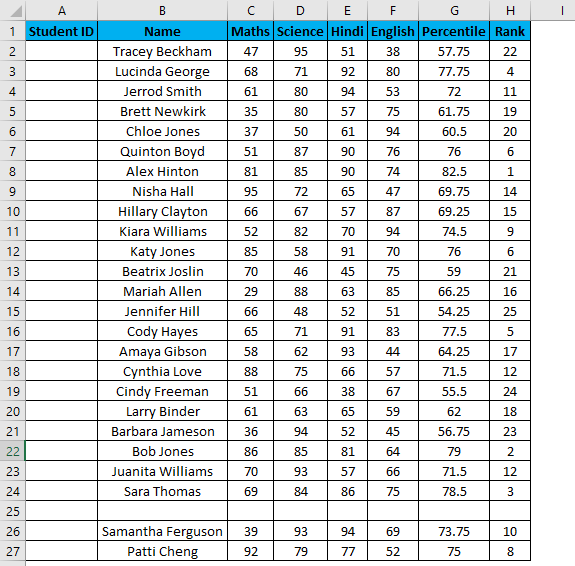
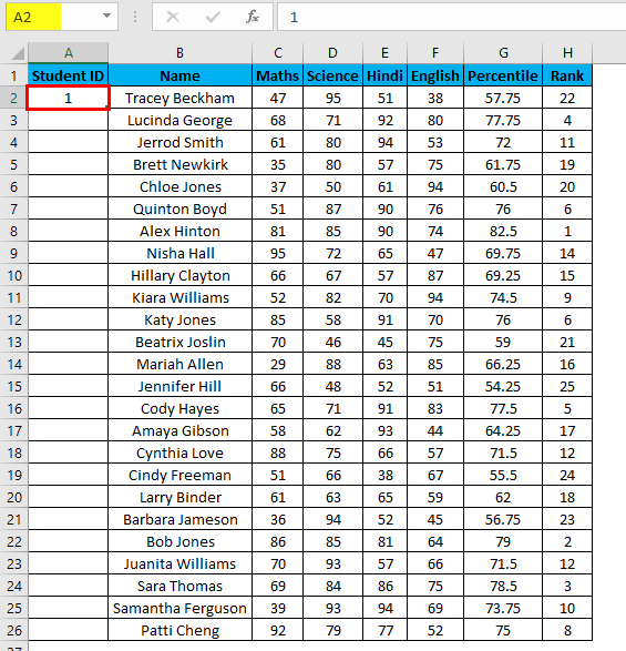
Suppose you have the following dataset. And you have to give a Student ID to each entry. Student ID there will be the same as the serial number of each row entry.
You can use the fill-handle method here.
For example, you want to give Student ID 1056 to the first student, and after, it should be numerically increasing, 1056, 1057,1058, and so on…
Steps to number rows in Excel:
- Enter 1056 in cell A2 and 1057 in cell A3.
- Select both cells.
- Now you can notice a square at the bottom-right of selected cells.
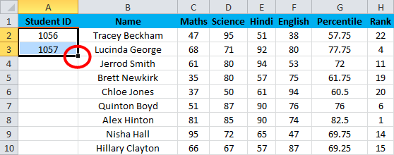
- Move your cursor to this square; now, it will be changed to the small plus sign.
- Now double-click this plus icon, and it will automatically fill the series till the end of the dataset.
Key Point:
- It identifies a pattern from a few filled cells and quickly fills the selected column.
- Viz. If you have any blank row(s) between your dataset. It will not detect them, so using the fill method is not recommended. It would only work till the last contiguous non-blank row.
Example #2 – Fill Series Method
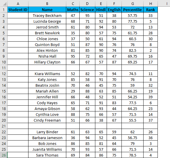
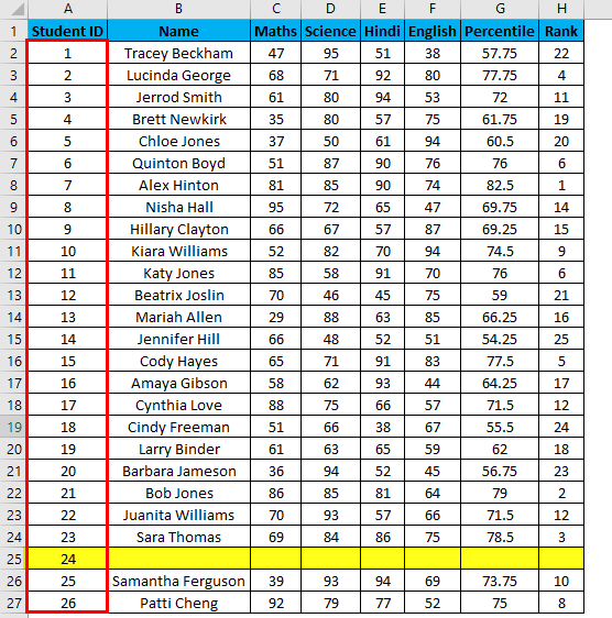
Suppose now we have the following dataset (same as above, now entries are only 26.).
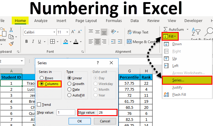
Steps to use the Fill Series method:
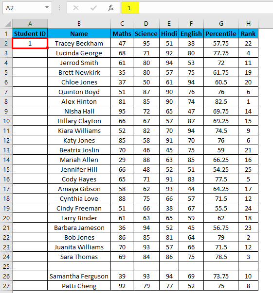
- Enter 1 in cell A2.
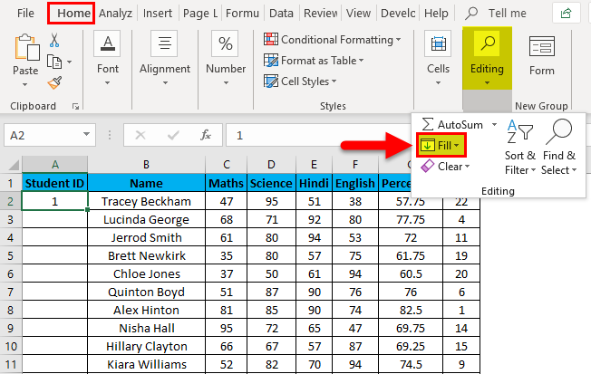
- Go to the Home tab.
- In the Editing group, click on the Fill drop-down.
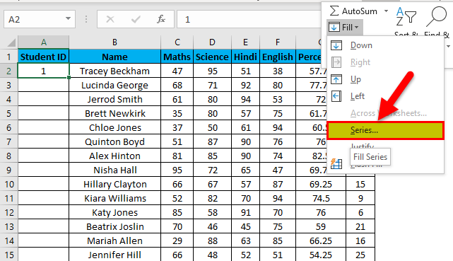
- From the drop-down, select Series.
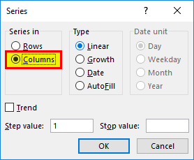
- In the Series dialog box, select Columns in the “Series in “option.
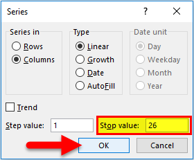
- Specify the Stop value. Here we can enter 26 and then click Ok.
- If you don’t enter any value, Fill Series will not work.
Hotkey to use fill series: ALT key+ H+ FI+ S
You can notice it overcomes the drawback of the previous method. But then it has its own drawback: if we have blank rows between the dataset, Fill Series would still fill the number for that row.
Example #3 – COUNTA Function
Suppose you have the same data set as above now if you want to number rows in Excel only which are filled Viz. Overcoming the shortcomings of the above 2 methods. You can use a COUNTA function here.
Steps to using a COUNTA Function:
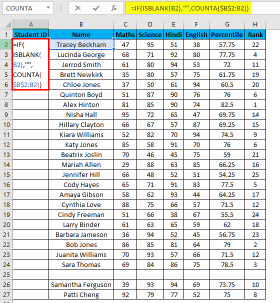
- Now enter the formula in the cell A2 i.e. =IF(ISBLANK(B2),””,COUNTA($B$2:B2))
- Drag it down till the last row of your data set.
- In the above formula, the IF function will check whether cell B2 is empty. If found empty, it returns a blank, but it returns the count of all the filled cells till that cell if it’s not.
Example #4 – Increment Previous Row Number
This is a very simple method. The main method is to add 1 to the previous row number simply.
Suppose you again have the same dataset.
- In the first row, manually enter 1 or any number from where you want to start numbering all rows in Excel. In our case. Enter 1 in cell A2.
- Now in cell A3, simply enter the formula=A2+1.
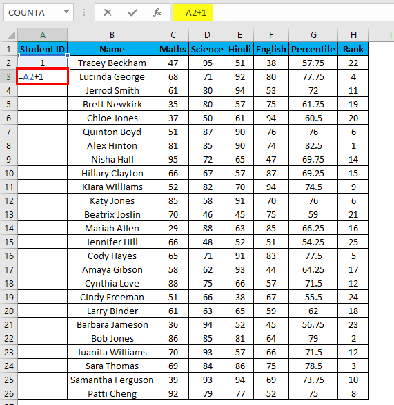
- Drag this formula until the last row, and it will be increased by 1 in each following row.

Example #5 – Row Function
In all methods, the serial number inserted is a fixed value. We can even use a row function to give serial numbers to rows in our columns. But what if a row is moved or you cut and paste data somewhere else in the worksheet?
The above problem can be resolved by using the ROW function. To number the rows in a given dataset using the ROW function.
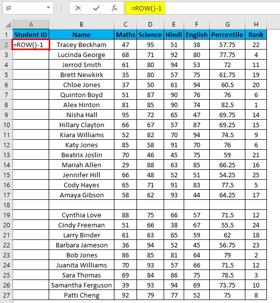
- Enter the formula in the first cell i.e. =IF(ISBLANK(B2),””,ROW()-1)
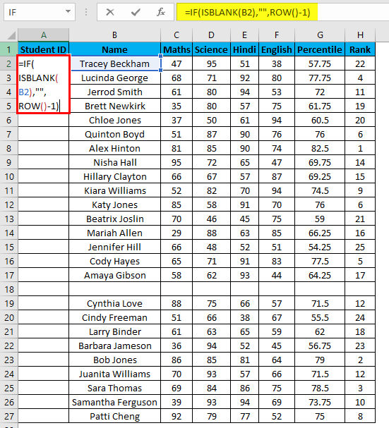
- Drag this formula until the last row.
- The above formula IF function will check if the adjacent cell B is blank. If it’s found blank, it will return space, and if non-blank, then the row function will come into the picture. The ROW() function will give us the row number since the first row in Excel consists of our dataset. So we don’t need to count it. To eliminate the first row, I have subtracted 1 from the returned value of the above function.
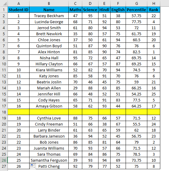
- But it will not still adjust the row number, and a blank row will still have a serial number assigned to it. Though it is not shown, look at the below screenshot.
- You can overcome the above issue with this formula, i.e.=ROW()-1
- Drag this formula until the last row.
- But now, it will consider the dataset’s blank rows and number them as well. Consider the below screenshot.

The main advantage of using this method is even if you delete one or more entries in your dataset. You don’t need to struggle with the numbering of rows each and every time, and it will be corrected automatically in Excel.
So by now, I have discussed 5 unique methods to give serial numbers to rows in a dataset stored in Excel. Although there are numerous methods to do the same, the above five are the most common and easy to use methods that can be implemented in different scenarios.
Things to Remember About Numbering in Excel
- While storing data in Excel, we often need to give serial numbers to each row in our data set.
- Entering a serial number in each and every row in the huge dataset can be time-consuming and prone to error.
Recommended Articles
This has been a guide to Numbering in Excel. Here we discuss how to add serial Numbers using different Excel methods, practical examples, and a downloadable Excel template. You can also go through our other suggested articles –
