Updated August 10, 2023
ROW in Excel
Row function in excel is used to get the row number of any selected cell irrespective of the values in a selected reference cell. To use the Row function, we just have to select the cell whose row number we want to identify; in return, we will have the row number of those reference cells. We can either select the row number or the cell whose row number we need to know.
ROW Formula in Excel
Below is the ROW Formula in Excel :
The ROW Function in Excel has the below-mentioned arguments:
- [reference] : (Optional argument): The range of cells or cell reference for which you want the row number. The ROW function always returns a numeric value
Note:
- If the [reference] argument is left blank or not entered or omitted, then the function returns the row number of the current cell (i.e. It is the cell where the row function is entered).
- Multiple references or addresses can be added or included in the ROW function.
- If the reference argument is entered as an array, then the ROW Function in Excel returns the row numbers of all the rows in that array.
How to Use the ROW Function in Excel?
The ROW Function in Excel is very simple and easy to use. Let us now see how to use this ROW Function in Excel with the help of some examples.
Example #1 – To Find out the ROW Number of the Current Cell
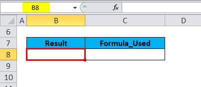
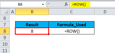
If you enter =ROW() in any cell in Excel, it will return the cell’s row number. Let’s check out this. In the below-mentioned example, For Cell “B8”, I need to find out the row number of that cell with the help of the ROW function.
Let’s apply the ROW function in cell “B8”, Select the cell “B8” where the ROW function needs to be applied.
Click the insert function button (fx) under the formula toolbar; a dialog box will appear, type the keyword “row” in the search for a function box, ROW function will appear in the select a Function box. Double-click on the ROW Function.
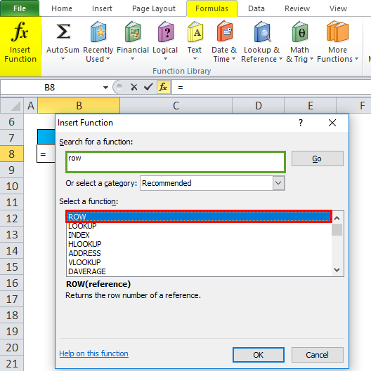
A dialog box appears where arguments for the ROW function need to be filled or entered, i.e. =ROW([reference]).
[reference]: (Optional argument) It is a cell reference for which you want the row number. Here it is left blank, or this argument is not entered because we want the row number of the current cell (i.e. It is the cell that the row function is entered into). Click OK.
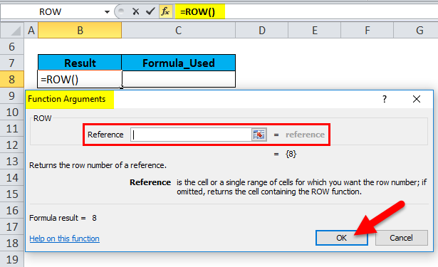
=ROW() without reference argument returns the row number of the cell where you entered the row function, i.e. 8.
Example #2 – To Find out the ROW Number of the Specified Cell
If you mention a cell reference with the ROW function, it will return the row number of that cell reference. Let’s check out this here.
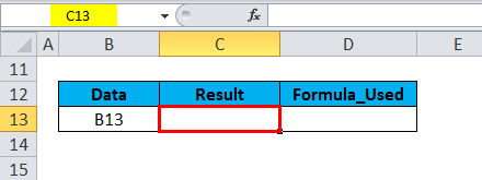
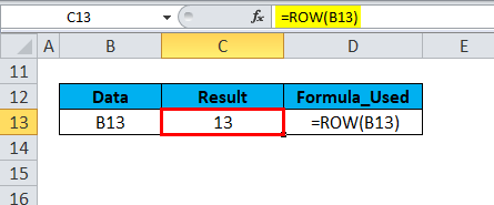
In the below-mentioned example, the Data column contains “B13” in the cell B13; I need to find out the row number of that cell with the help of the ROW function.
Let’s apply the ROW function in cell “C13”, Select the cell “C13” where the ROW function needs to be applied.
Click the insert function button (fx) under the formula toolbar; a dialog box will appear, type the keyword “ROW” in the search for a function box, and the ROW function will appear in the select a Function box. Double-click on the ROW function.

A dialog box appears where arguments for the ROW function need to be filled or entered, i.e. =ROW([reference])
[reference]: It is a cell reference for which you want the row number. Here it is, “B13”. Click ok. after entering the reference argument in the row function, i.e. =ROW(B13).
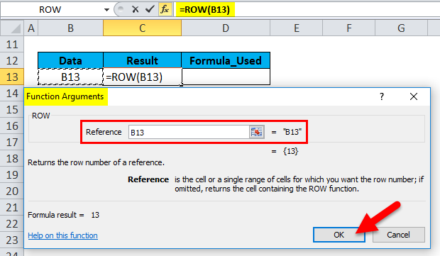
=ROW(B13) returns the row number of that specified cell reference, i.e. 13.
Example #3 – To Find out ROW Numbers for a Range of Cells
When we apply the Row function for a specified range in Excel, it will return the row number of the topmost row in the specified range; let’s check out this here.
In the below-mentioned example, the Table contains the student score in column F & their subject score in column G. It’s in a range of F7:G11; I need to find out the topmost row in the specified range (F7:G11) with the help of the ROW function.
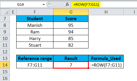
Let’s apply the ROW function in cell “G14”, Select the cell “G14” where the ROW Function needs to be applied.

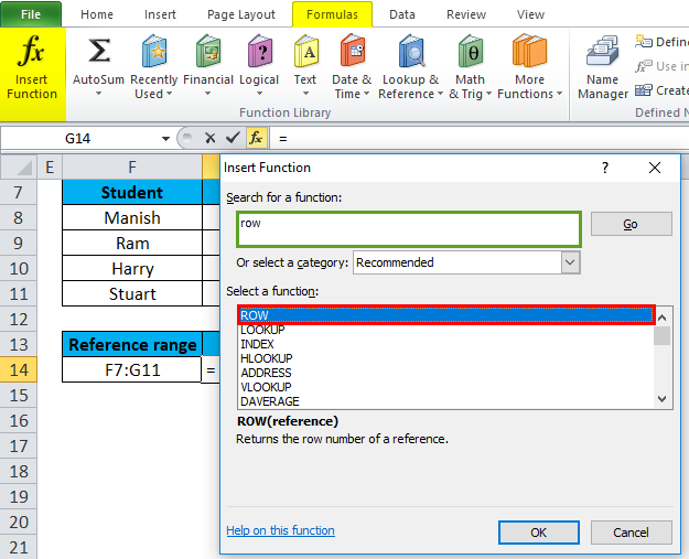
Click the insert function button (fx) under the formula toolbar; a dialog box will appear, type the keyword “row” in the search for a function box, ROW function will appear in the select a Function box. Double-click on the ROW function.
A dialog box appears where arguments for the ROW function need to be filled or entered, i.e. =ROW([reference])
[reference]: is a cell or range of cells for which we want the row number.
Here we are taking input reference as a range of cells, i.e. F7:G11. Click ok. after entering the reference argument (F7:G11) in the row function, i.e. =ROW(F7:G11).
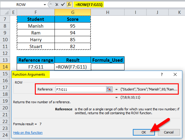
=ROW(F7:G11) returns the row number of the topmost row in the specified range, i.e. 7.
Things to Remember about the ROW Function in Excel
- The ROW Function in Excel accepts an empty value, reference & range values in the argument.
- The ROW function argument is optional, i.e. =ROW([reference]). Whenever there is a square bracket [] in an argument of Excel function, it indicates that the argument is an optional parameter, which you can skip or leave blank.
- Row Function is used as a nested function with other Excel functions, i.e. It is commonly used along with other Excel functions like ADDRESS, IF (Logical functions) & other functions with multiple criteria.
- ROW Function has limitations; ROW Function considers only one input, so we cannot enter multiple references or addresses in a row argument.
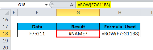
- In the ROW Function, we can enter the arguments’ cell references or range values. If we try to use or add any of the other references along with that range, will the ROW Function return an #NAME? error.
In the below-mentioned example, Here I have added “B8” cell reference along with range value “F7:G11”, i.e. =ROW (F7:G11B8)
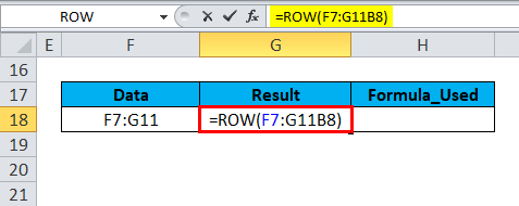
=ROW (F7:G11B8) will result in or returns #NAME? error.
Recommended Articles
This has been a guide to ROW in Excel. Here we discuss the ROW Formula in Excel, how to use a ROW Function in Excel, practical examples, and a downloadable Excel template. You can also go through our other suggested articles –
