What is a MODE in Excel?
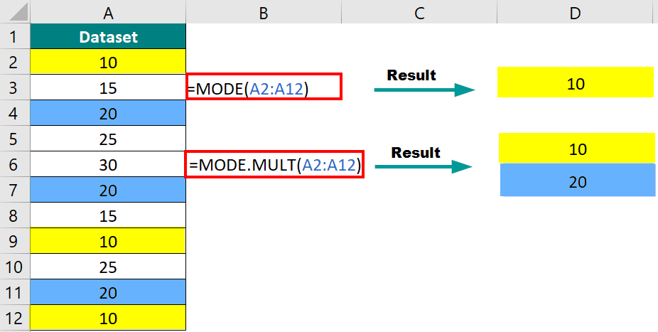
MODE in Excel is a statistical function that helps you find which value appears most frequently in a range of data. For instance, if you have a dataset with the numbers 5, 4, and 5. In this case, MODE in Excel will give the result as 5 since it appears most frequently (twice).
The MODE function in Excel can be particularly useful when working with a large dataset and you want to identify the most common value.
Syntax
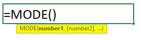
In the Syntax,
- number1: The first number or range for the dataset.
- number2, [number3], … (Optional): Additional numbers or cell references for the dataset.
Table of Contents
How to Use MODE in Excel?
In some datasets, there can be more than one mode value. That is, two, three, or more values (number or text) appear a maximum number of times. Thus, some datasets have only one mode value (single), and others have more than one (multiple).
- MODE Function (To find Single Mode Value)
- MODE.SNGL (To find Single Mode Value)
- MODE.MULT (To find Multiple Mode Value)
- Pivot Table (To find Multiple Mode Value)
1. MODE in Excel
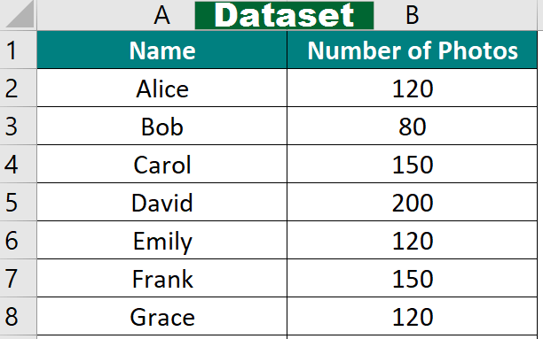
Let’s consider an example involving the number of vacation photos people took during their trips. We need to find which value for the number of photos occurs more than once.
Given:
Solution:
Step 1: Select a cell where you want to display the result, cell B9.
![]()
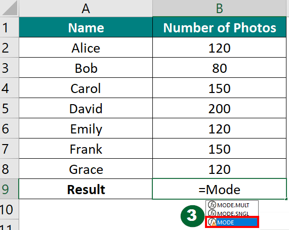
Step 2: In the selected cell (B9), enter the formula: =MODE.
![]()
Step 3: Select MODE by double-clicking from the given options.
Step 4: Select the range B2 to B8 as the input, which contains the number of photos taken.
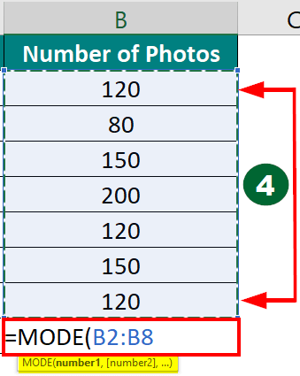
Step 5: Press Enter. The result in cell B9 will be the mode (the most frequently occurring value in the dataset).
![]()
Result:
The mode preferred number of photos taken is 120 because it appears thrice in the dataset (Alice, Emily, and Grace).
2. SNGL Function Using Excel Ribbon
You can also use the MODE function in Excel using Ribbon. Let us use the same example given above and try to find the mode value using the Excel ribbon. However, we made a small change. The number for Grace is now 80.
Step 1: Select the cell (B9) where you want the result (the mode) to appear.
Step 2: Go to the “Formulas” tab on the Excel ribbon.
Step 3: In the “Function Library” group, click on the “More Functions” dropdown (small inverted triangle).
Step 4: Select “Statistical” and then choose “MODE.SNGL.”
Step 5: Once the “Function Arguments” dialog box appears,
- For the “Number1” field, select the range of cells that contain your data (e.g., B2:B8 if your data is in column B from rows 2 to 8).
- Leave the “Number2”, “Number3”, etc., fields empty, as you work with a single range.
Step 6: Click the “OK” button.
Result:
The MODE function will display the result (120) in the selected cell.
3. MODE.MULT Function in Excel
We can also use the MODE function using Insert Function from the Formula tab. Let us use this method to see how we can find a mode for multimodal data (the dataset that has more than one mode value).
Let’s say we have a dataset that represents the scores of students in a class on a recent math quiz. We want to find the mode value for the scores.
Step 1: Select the cell where you want the results to appear. Let’s use cell D3.
Step 2: Go to the “Formula” tab in the Excel ribbon.
Step 3: Click on the “Insert Function” button. It looks like fx and is usually present at the left of the formula bar. A dialog box for “Insert Function” will open.
Step 4: From the list of functions that appear, select “MODE.MULT,” present under the “Statistical Functions,” and click “OK.”
Step 5: A dialog box named “Function Arguments” appears for the MODE.MULT function.
Step 6: In the “Number1” field, select the range of data for which you want to find the modes. Select the range B2:B9 in this example and click “OK.”
Step 7: Excel will display the results in the selected cells.
Step 8: Now, double-click on the first cell (D3) and press Ctrl+Shift+Enter. The array formula will now be enclosed in curly braces like this: {=MODE.MULT(B2:B9)}.
4. MODE using Pivot Table
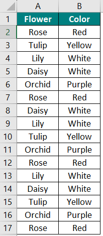
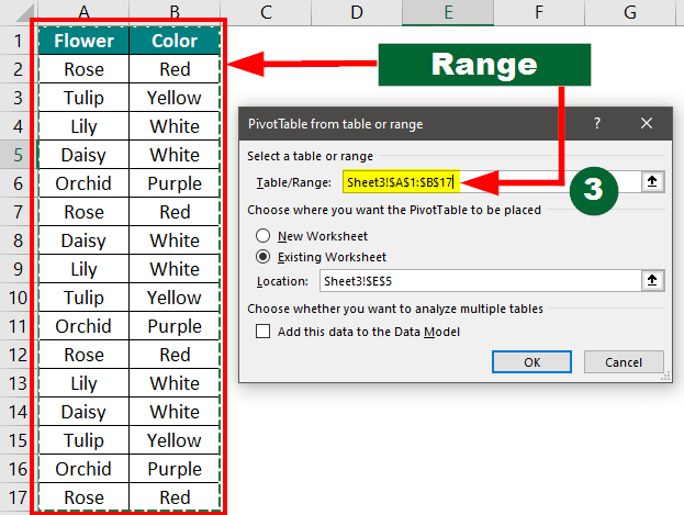
Suppose you have two columns, “Flower” and “Color,” and want to find all the mode values in the data and the number of times they appear. Let us use the pivot table to find the mode values.
Given:
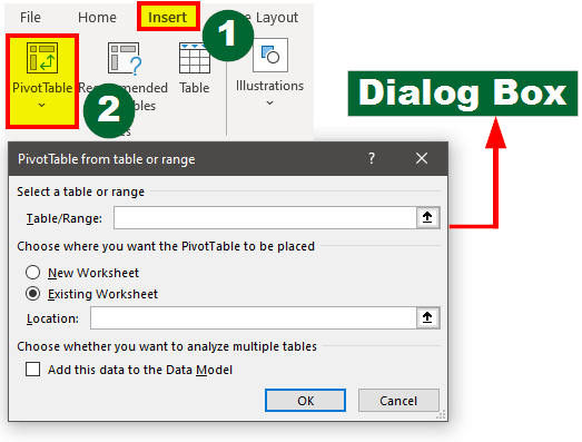
Step 1: Go to the “Insert” tab in the Excel ribbon
Step 2: Click “PivotTable” from the “Tables” group. The PivotTable dialog box will appear.
Step 3: Verify that the “Select a table or range” option displays your data range correctly. If not, click and drag to adjust the content to cover your data.
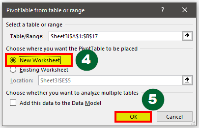
Step 4: Choose the “New Worksheet” option to place the Pivot Table in a new sheet
Step 5: Click “OK.”
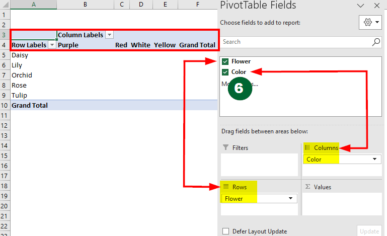
Step 6: In the new worksheet, you’ll see the “PivotTable field” on the right side.
In the field list,
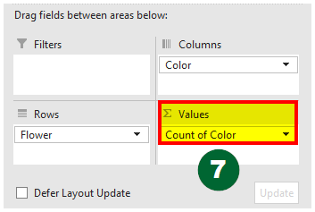
- Drag the “Flower” field to the “Rows” area
- Drag the “Color” field to the “Columns”
This will list unique flower names and colors in respective rows and columns.
Step 7: Again, drag any field (e.g., “Color” or “Flower”) to the “Values” area. Excel will automatically count the times that each color occurs in the dataset.
Result:
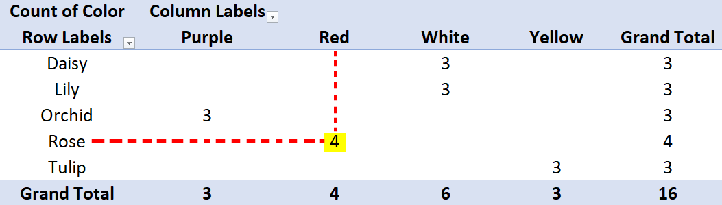
In the Pivot Table, you will see the flower names in rows and colors in columns. The cells where flower names and colors meet display how often the combination occurs.
For instance, the cell where “Rose” and “Red” intersect in the below image has the highest count, “4.” Hence, “Rose” with the color “Red” is the mode flower-color combination in the dataset.
Things to Remember
- MODE shows the #N/A error value if there are no duplicates in the data.
- Arguments can be numbers or names, references, or arrays containing numbers.
- If you are unsure whether there is more than one mode in your data, you can use the MODE.MULT function to see all the mode values. You can check example 3 of this article.
Frequently Asked Questions (FAQs)
Q1. Which functions in Excel can you apply the MODE function to?
Answer: We can use the MODE in Excel with several other Excel functions such as IF, SUMIF, and COUNTIF to count the occurrences of each unique value or find the sum of those values. We can also use the MATCH function to find information for a specific item.
Q2. What is the purpose of using the mode formula in Excel?
Answer: The mode formula in Excel helps find the most frequent value in a data set. It can help businesses find which value occurs most frequently and make decisions accordingly.
For example, if a company takes a survey from 100 people on which product they like the most. The company can then use MODE in Excel to find which product’s name occurs most frequently. This way, they can identify their best-selling product.
Recommended Articles
This is a detailed guide on MODE in Excel. We explain the 4 methods in which you can use the MODE function in Excel to find the mode values. Visit the following articles for more Excel-related information.