Updated July 5, 2023
Group in Excel
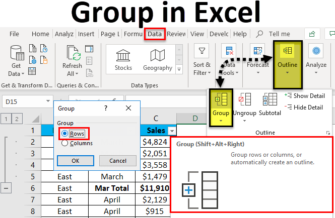
Use grouping in Excel when you have properly structured data and mention the header names in the column. There, grouping allows users to club rows or columns of any number together so that we can hide or, in proper words, subset the data under the selected columns and rows. To access Group in Excel, go to the Data menu tab and select the Group option. Then select the row or column which we want to select. Suppose we select 5 rows in a sequence; then we can use the plus sign, which is used to expand or collapse the selected rows.
Group and Ungroup Command (Keyboard shortcut in Excel)
Group: Press Shift + Alt + Right Arrow shortcut rather than going to the data tab, then clicking the group button and selecting the row or column option.
Ungroup: Press Shift + Alt + Left Arrow shortcut rather than going to the data tab, then clicking the ungroup button and selecting the row or column option.
How to Create a Group in Excel?
Creating a group in Excel is very simple and easy. Let’s understand how to create a group in Excel with some examples.
Example #1 – Group for Row
Step 1: Now, look at the below data in Excel Sheet which a user wants to be grouped.
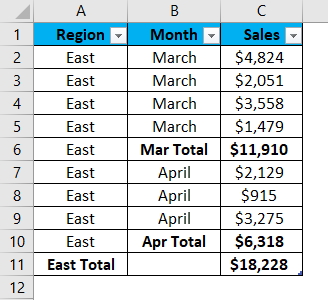
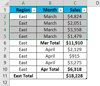
Step 2: Select all row that needs to be in one group (As we can see, the user is selected for March month data from the table)
Step 3: Now go to the Data menu bar. Click on Outline and then click on the Group toolbar.
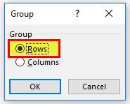
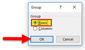
Step 4: The pop- up Group will now show that select Rows (As the user wants to group by row).
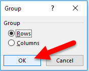
Step 5: Now click on the OK button.
Summary of Example 1: As the user selects the row for the month of March, it is grouped into one. As well as two-level buttons are created on the left of the worksheet, the highest level, level 2, will show all the data, while level 1 will hide the details of each size and leave subtotal.
Now the user can hide or show the group using the button attached to the bracket on the left side. Click the minus sign to hide, and the plus sign to show it again.
Example #2 – Create a Nested group
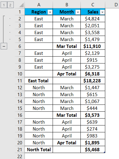
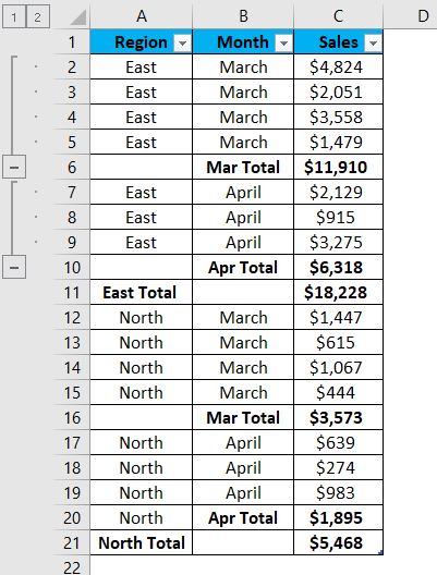
Step 1: Look at the below data in Excel Sheet, which a user wants to group, and select the row/column.
Step 2: The user has selected a row for March, and the region is East. Now go to the Data menu bar. Click on Outline and then click on the Group toolbar.
Step 3: Now Group pop-up will appear, select Rows and click Ok.

The very first group will be created.
Step 4: Now select the April month data for the same region. Now go to the Data menu bar. Click on Outline and then click on Group.
Step 5: Again, a Group pop-up will appear, select Rows and click Ok.
Now the second group will be created.
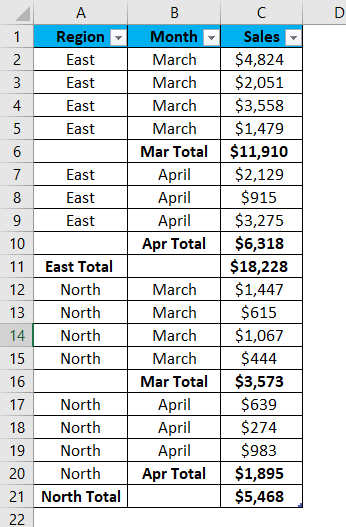
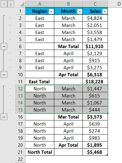
Step 6: Similarly, select the north region and create a group. Now the 3rd group will be created.
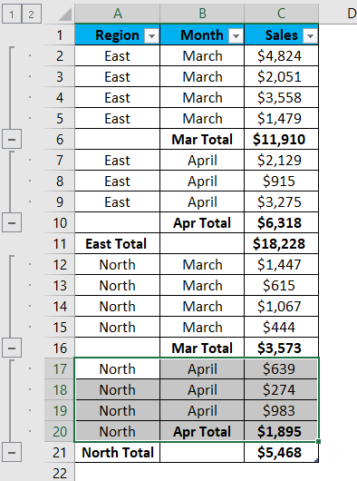
In the same way, the 4th group is also created.
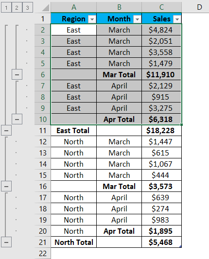
Step 7: Select the entire eastern region row, and the 5th group will be created.
Step 8: Select the entire north region row, and the 6th group will be created.
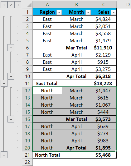
Summary of Example 2: As the user selects a row for each month, it is grouped into one. As well as three-level buttons are created on the left of the worksheet; the highest level, level 3, will show all of the data, while level 2 will hide the details of each region and leave subtotal. Finally, level one will take a grand total of each region.
Now the user can hide or show the group using the button attached to the bracket on the left side. Click the minus sign to hide, and the plus sign to show it again.
Example #3 – Group for Worksheet in Excel
Step 1: Go to Sheet Q1 in Excel Sheet, where the user wants to group with Q2 and Q3.
Step 2: Select the Q1 sheet and press the Ctrl button. Along with that, select all sheets in which the user wants to be in one group (As we can see, the user has selected Q1, Q2, and Q3 from the worksheet)
Step 3: Now release the Ctrl button, and all three sheets will be grouped.
Summary of Example 3: The Q1, Q2, and Q3 sheets the user selects will be grouped. Now a user can perform an edit on multiple sheets at the same time.
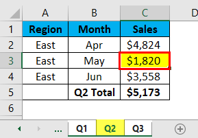
Let’s take an example where a user wants to update the data for August in the East region from Q3 sheets to $1820.
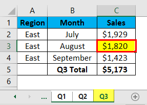
Go to the other sheet; each sheet will update this value.
Uses of Group in Excel
- We used to get a worksheet with a lot of complex and detailed information, and it is very hard to understand something quickly, so the best way to organize or simplify our worksheet is by using Group in Excel.
- The user needs to make sure whenever they are going to use a group; there should be a column header, a summary row, or a subtotal; if it is not there, then we can create it with the help of the subtotal button, which is available in the same toolbar of group button.
- In Excel, a user should never hide cells because it will not be clear to the other users that cells are hidden so that they can be unnoticed. So, using a group here rather than hiding cells is best.
Things to Remember
- If the user wants to ungroup, select the row or column, go to the Data menu bar, and click the Ungroup button.
- Always ensure whichever column a user wants to make a group has some label in the first row, and there should be no blank row or column in Excel.
- While creating a group, ensure all data are visible to avoid incorrect grouping.
- Removing the group will not delete any data in Excel.
- Once the user ungroups or groups, he can reverse by Undo button (Ctr+Z).
- It is impossible to ungroup other adjacent groups of columns /rows simultaneously; the user must do it separately.
Recommended Articles
This has been a guide to Group in Excel. Here we discuss its uses, how to create Group in Excel, practical examples, and a downloadable Excel template. You can also go through our other suggested articles –
