Updated June 8, 2023
FV Formula in Excel
FV Formula in Excel or the Future Value formula calculates the future value of any loan amount or investment. FV Formula returns the future value of any loan or investment considering the fixed payment that needs to be done for each period, the rate of interest, and the investment or loan tenure.
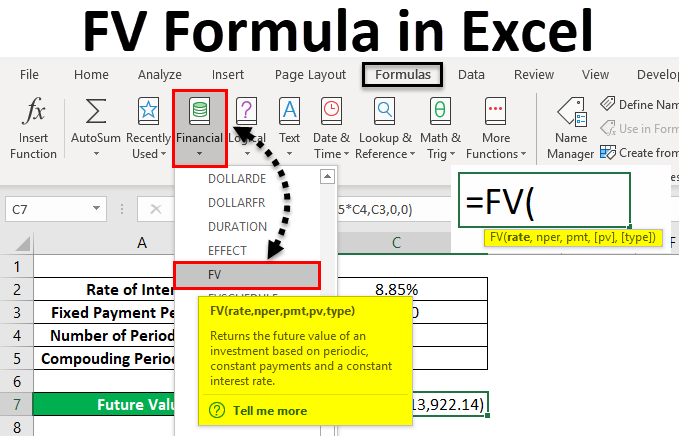
FV Formula in Excel can be used from Insert Function beside the formula bar by clicking the icon.
FV Formula in Excel has the following arguments:
- Rate: It is the rate of interest per compounding period. We can directly use the whole interest rate or divide this with the total compounding period, say, a month, and use the interest applied for a single month.
- Nper: It can be monthly, quarterly, or yearly, depending on how the customer opts for the payment term. Nor is the total number of payments or the installments of the whole tenure.
- Pmt: It is a fixed amount we must pay in a period.
The above-shown arguments are mandatorily required in FV Excel Formula. Below are some optional arguments as well;
- Pv: It is the present value of an asset or investment. Suppose we bought a vehicle 2 years back. So at present, whatever will be its market value will be kept here. If we do not keep this value, it will automatically be considered 0.
- Type: Use 1 if the EMI is paid at the start of the month and 0 if the EMI is paid at the end of the month. For this, if we do not keep them in Excel automatically, it will be considered as 0.
How to Use FV Formula in Excel?
The FV formula in Excel is very simple and easy to use. Let’s understand how to use FV Formula in Excel with some examples.
Excel FV Formula – Example #1
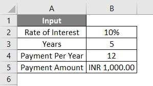
We have data where a person wants to make some investment. The Investment Company is offering a return interest rate of 10% yearly. And that person opts for 5 years with a fixed monthly payment of nearly Rs. 1000/- plan.
If we summarize the above data, then we will have the following;
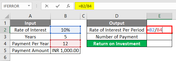
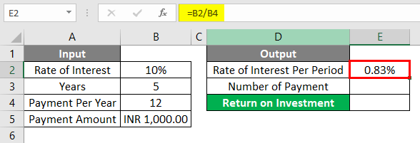
As we have discussed in the argument above so, we can keep a rate of interest as it is, or we can divide it within the formula, or else we can first scrub the argument separately and then use it in the formula. For better understanding, first, let us scrub the data separately. For that, we need a rate of interest applicable per month which will be our Rate, and the total number of payments that will be made in the whole tenure of the loan, which will be our Nper.
As per the Input data we have seen above, our Rate is calculated using the formula =B2/B4.
The Result will be as given below.
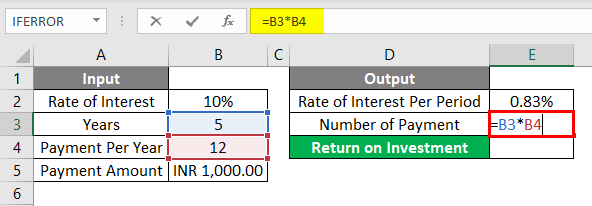
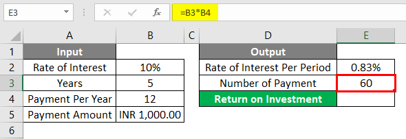
Nper is calculated by using the formula =B3*B4
The Result will be as shown below.
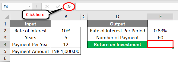
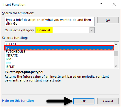
Now we can directly use these parameters in our Excel FV Formula. First, go to the cell where we need the output. Then go to the insert function option beside the formula bar, as shown below.
Once we do that, we will get the Insert function box. Now from there, under the Financial category from Or select a category option, search FV function from the list. Or else, we can keep the Or select a category as ALL and look for the required function as shown below. And click on Ok.
Now for the selected cell for output E2, we will get an argument box for FV Function. From there, select the Rate, Nper, and Pmt calculated above.
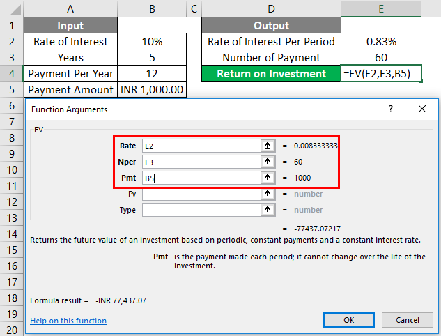
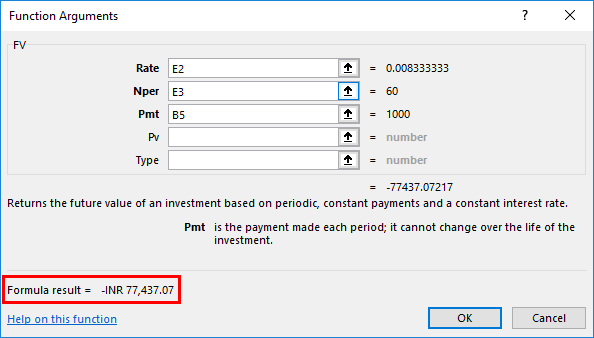
We have selected all the necessary cells for the function argument of the FV Formula. At the bottom left of the argument box, we will get the result of the applied function. Here we are getting the result negative, which means the invested amount granted from the bank.
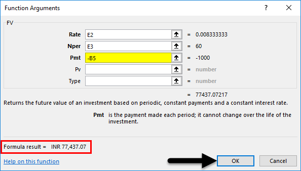
If we need to use this data in another form, we can apply a negative sign’ -‘ in the Pmt argument box to get a positive result. And once we apply the negative signs, we will see the positive formula result in the bottom left of the argument box. Once done, click on Ok.
Once we click Ok, we will get the result in the selected cell, as shown below.
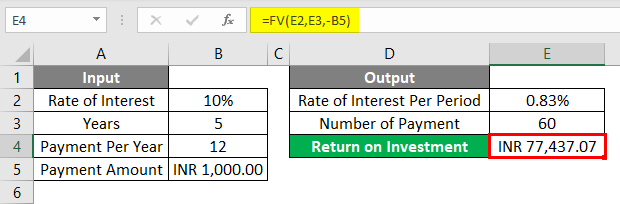
The calculated future value of invested amount, which is in INR (Indian Rupees) as Rs. 77,437.07/-, is the final amount that that person can gain for 5-year tenure with an interest rate of 10% if that person pays Rs. 1000/- monthly EMI as an investment for 5 years.
Excel FV Formula – Example #2
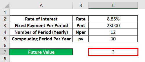
Below is another example for which we need to calculate the Future Value or compounded Loan amount.
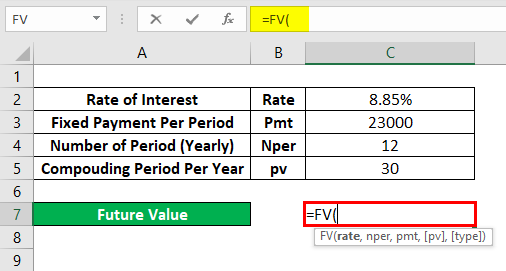
For this, go to the edit mode of the cell, where we need to see the output by typing the “=” sign (Equal). And search and select FV Formula in Excel as shown below.
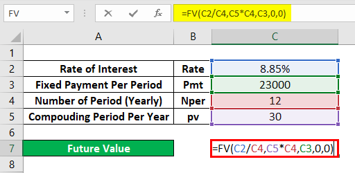
Here we will directly use the data and crunch it in the formula, as shown below. We have divided the Rate by the total number of months of the loan period. And Nper will multiply 12 and 30 as a compounded period. And we have considered the compounding period amount as Rs 23000/-, which is our PV.
Now press the Enter key to get the result, as shown below.
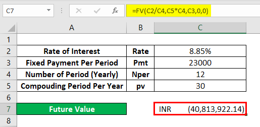
As the obtained value FV is Rs. 40,813,922.14/- which means the future value of the loan amount after 30 years of compounding will be Rs. 40,813,922.14/-
Pros
- It is quite useful in most financial calculations.
- Because of ease of use, anyone can calculate their return on investment.
Things to Remember About FV Formula in Excel
- A negative sign used in example-1 shows the amount invested by the customer through an investment firm.
- Keeping “0” for Type means that EMI payments are made at the end of the month.
- You should consider PV (Present value) in some cases where the compound interest rate applies.
Recommended Articles
This has been a guide to FV Formula in Excel. Here we discuss how to use the FV formula in Excel, practical examples, and a downloadable Excel template. You can also go through our other suggested articles –
