Updated May 8, 2023
Introduction to NPER in Excel
The NPER function in Excel determines how many payments a customer needs to make for the borrowed loan or invested amount. And those numbers of payments (NPER) will be based on a fixed amount to be paid at the current interest rate. This also has the option of whether payment will be made at the start or the end of the month.
Syntax
An argument in the NPER Formula
- rate is required to specify the interest rate per period.
- pmt – is a required argument that specifies the amount paid at each period which contains the principal amount and interest rate (excluding taxes and other fees).
- pv – is a required argument that is nothing but the actual loan amount.
- fv – an optional argument that specifies the future value of the loan amount.
- type – the optional argument specifying whether the payment is to be made at the start or at the end of the period: 0 – payment made at the end of the period, 1 – payment made at the start of the period.
How to Use Excel NPER in Excel?
NPER in Excel is very simple and easy. Let’s use the NPER in Excel with a few examples.
Example #1 – NPER Simple Example in Excel
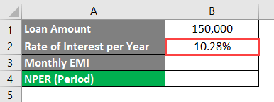
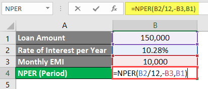
Mr. Akshay has taken a loan of 1,50,000 for higher studies. He agreed to pay the amount with a rate of interest of 10.28% per annum and can pay 10,000 per month. However, he is still determining when he can clear the loan amount. We will help him to find this out with the help of the NPER function in Microsoft Excel.
In cell B1, the value of the Loan Amount.
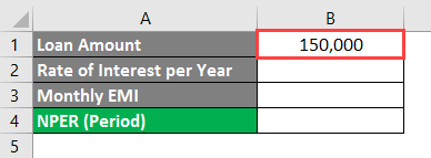
In cell B2, Input the Rate of Interest per Year Value (10.28% in the case of Mr. Akshay).
In cell B3, the value of the Monthly EMI that Mr. Akshay can pay on behalf of his Loan Amount.
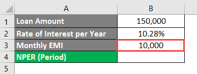
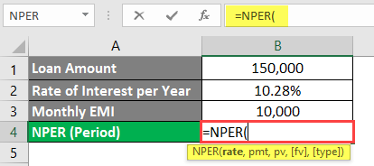
We need to find out the period under which Mr. Akshay can pay this amount with a monthly EMI of 10,000 and a rate of interest of 10.28% per annum. This value we need to calculate in cell B4.
In cell B4, start typing the formula of NPER.
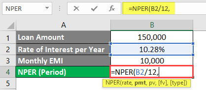
Mention B2/12 as the first argument for the NPER formula. As a given Rate of Interest is per year, we need to break it down to the monthly interest rate because we are paying the amount per month.
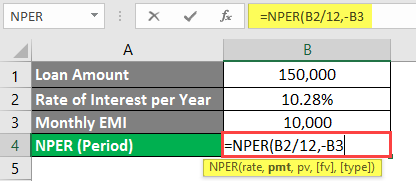
The next argument is the amount to be paid at each period; since Mr. Akshay is ready to pay the EMI amount of 10,000 per month (Cell B3), you will mention it as the next argument in the formula. However, please note that this amount is a cash outflow (an amount that will be deducted from Mr. Akshay’s account). Therefore, you need to mention it as a negative amount.
Input Mr. Akshay’s loan amount from the bank, i.e., 1,50,000 (stored in cell B1).
Press Enter key.
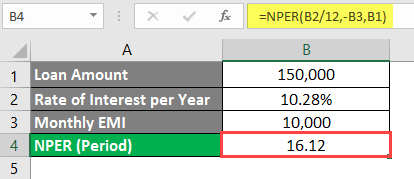
You can see that with the rate of interest of 10.28% per annum and monthly EMI of 10,000, Mr. Akshay can clear/repay his loan amount of 1,50,000 within 16.12 months.
Please note that in this formula, we have not included fv (future value of the loan) and type (whether the EMI is being paid at the start or the end of the month), as these are optional arguments.
Example #2 – Calculate Period for Future Value Increment
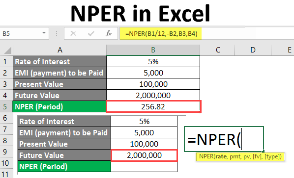
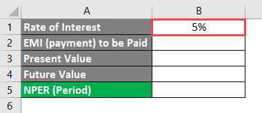
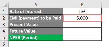
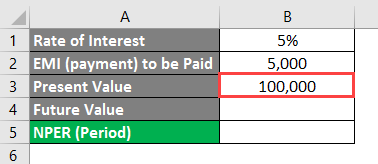
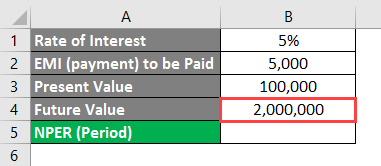
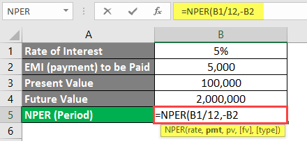
Mr. Sandeep, a 25-year-old engineer, wants to make some investments for his retirement. He wishes to have a lumpsum amount of 20,00,000 when he retires and is ready to invest 1,00,000 today (present value). We want to calculate the number of months Mr. Sandeep requires to earn 20,00,000. The yearly interest rate is 5%, and Mr. Sandeep is ready to pay a monthly EMI of 5,000.
In cell B1 of the Excel sheet, input the Annual Rate of Interest.
In cell B2, mention the payment amount Mr. Sandeep is ready to pay every month.
In cell B3, add the present value of the investment which Mr. Sandeep is about to make.
In cell B4, the future value will take place. The value which Mr. Sandeep wants is a lumpsum amount at the time of his retirement.
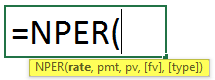
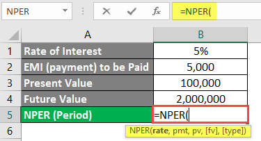
In cell B5, start typing the NPER Formula.
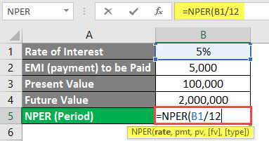
Put B1/12 as the first argument under NPER Formula. As the given interest rate is per annum, you need to divide it by 12 to get a monthly interest rate (because Mr. Sandeep is paying installments monthly).
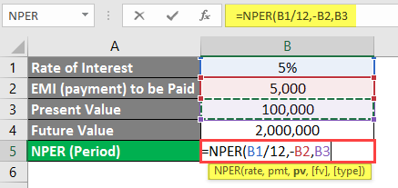
Mention -B2 as the next argument in this formula. As the value of 5,000 will be debited from Mr. Sandeep’s account (outgoing amount), we need to mention the negative sign.
The next argument would be the Present Value of the Investment in cell B3.
Lastly, mention B4 as an argument representing the Future Value of Investment.
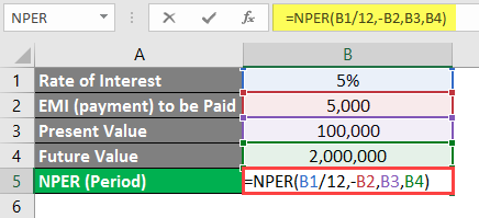
Press the Enter key, and you will get the number of months’ value; Mr. Sandeep has to make an investment to get 20,00,000 as a final amount when he retires.
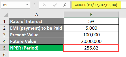
Here, if Mr. Sandeep makes a payment of 5,000 per month for the investment amount of 1,00,000, it will require 256.82 months (21.40 years) to get matured up to the lump sum of 20,00,000.
Things to Remember About NPER in Excel
- PMT under the NPER function generally includes interest amount. But not the taxes and additional processing fees.
- The rate of interest should be homogeneous throughout the period. For example, in the above examples, we have divided the yearly interest rate by 12 to make each month homogeneous throughout the year.
- The outgoing payments need to be considered debts and marked as negative payments.
- #VALUE! The error occurs when one of the required arguments from the formula is non-numeric.
- #NUM! An error occurs when the future value mentioned will not meet over the period of time with the mentioned rate of interest and EMI (investment amount). In that case, we need to increase the monthly investment amount. Also, this error occurs when outgoing payments are not marked as negative.
Recommended Articles
This is a guide to NPER in Excel. Here we discuss how to use NPER in Excel, practical examples, and a downloadable Excel template. You can also go through our other suggested articles –
