Excel AVERAGEIF

Excel AVERAGEIF (Table of Contents)

• Introduction to AVERAGEIF in Excel
• How to use the AVERAGEIF Function in Excel?

Introduction to AVERAGEIF in Excel

AVERAGEIF function in Excel is used to calculate the average of numbers based on defined criteria. For example, we have sales data of 4 product, and we want to find out the average sale of any product from the entire data or selected portion of data. For that, we use AVERAGEIF, whereas per syntax, we first select the range of all the products and then give select the criteria by selecting the product name for which we want to find average sale and then select the complete range of sold quantities.

Now, we have known the exact AVERAGEIF function; we will now learn how to write a formula using the formula’s function and syntax.

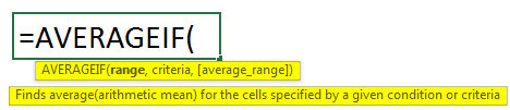
The syntax of the AVERAGEIF function

Here is the explanation of all the elements of the syntax.

• Range – A range of cells on which the criteria or condition is to be applied. The range can include a number, cell references and names as well. In case there is no “Average-range” argument, this range will be used for the calculation of average.
• Criteria – This is a condition based on which cells will be averaged. It could be a number, cell reference, text value, logical statement (like “<5”) or expression.
• average_range – The cell range to average. It is optional. In the absence of any average_range, the range is used to calculate the average.

How to use the AVERAGEIF Function in Excel?

Now, we will learn how to use the AVERAGEIF function in Excel with the help of various examples. It is an inbuilt function in Excel.

AVERAGEIF in Excel – Example #1

The AVERAGEIF function in Excel calculates the average of cells that exactly match the criteria or the condition specified.

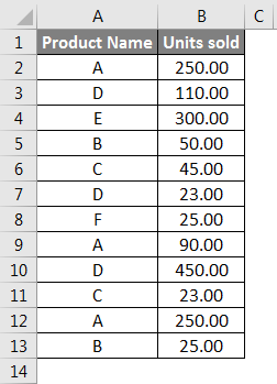
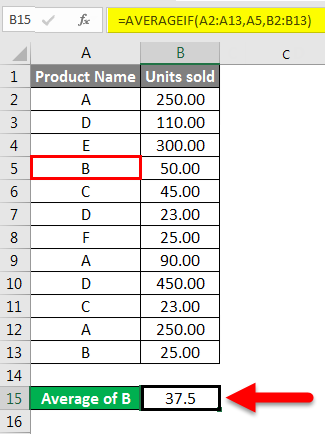
Below you will see a table containing the product name and the units that are sold.

In this example, we need to find the average units sold for product B.

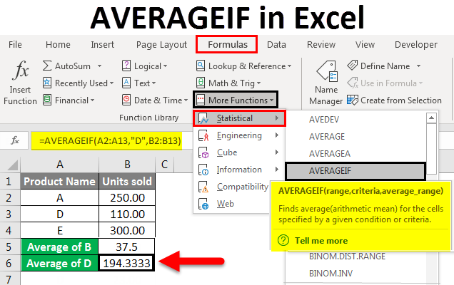
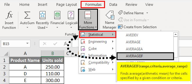
We can directly type the formula by starting it with = and typing AVERAGEIF, or we can also select the function from the ribbon as shown below:

Now Function Arguments Box will appear. Then select Range: A2:A13, Criteria: B15, Average_range: B2:B13.

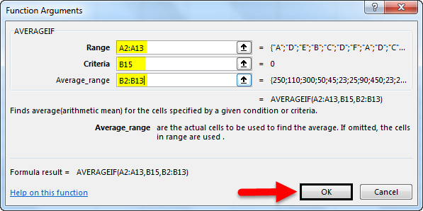
Press OK. We get the below result which is the average units sold for product B.

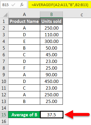
We can also type in “B” instead of cell reference in the formula as shown below in cell B15:

Explanation of the example :

Range: We have taken A2: A13 as the range on which our criteria (B) will be applied.

Criteria: Since we wanted to know the average units sold for B, so B is our criteria.

Average _range: B2: B13 is the range of cells from which Excel will do the average.

Taking our last example. Suppose we want to know the average units sold for D product.

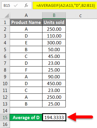
We will get the average units sold for D product = 194.33

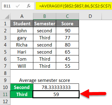
AVERAGEIF in Excel – Example #2

We have a sample data table that contains the score of students for the second and third semesters.

Now, if we want to calculate the average second-semester score from the above data, we can do it by writing the formula as shown below:

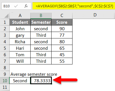
We will write B2:B7 as range and make it absolute by pressing F4. Then, we will write “second” as criteria and C2:C7 as average_range and make it an absolute range. We will get the average third-semester score by using cell reference B6 instead of the word “Third” as criteria.

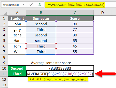
And we will press the Enter key to get the result.

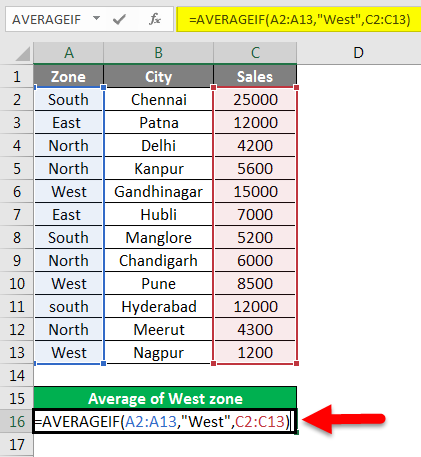
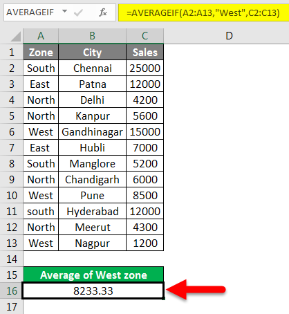
AVERAGEIF in Excel – Example #3

In this sample data, we have sales data for cities in different zones.

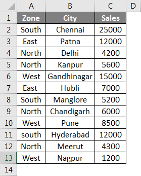
If we want to find the average sale of a particular zone, say, for instance, West. We can get average sales as below:

Press the Enter key to get the result.

So these examples must have given you a fair understanding of the use of the AVERAGEIF function.

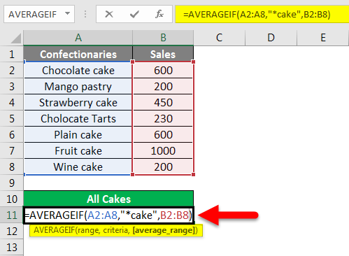
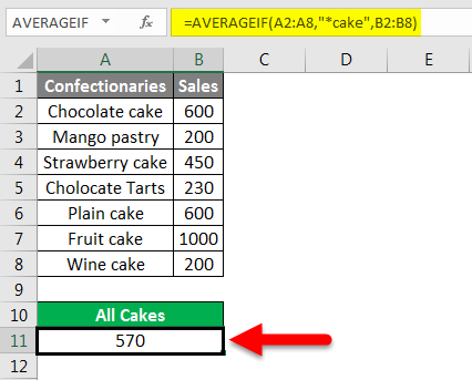
AVERAGEIF in Excel – Example #4

AVERAGEIF using a wildcard in-text criteria

We use a wildcard in the AVERAGEIF function when the text criteria are partially met or are preceded or followed by any other word.

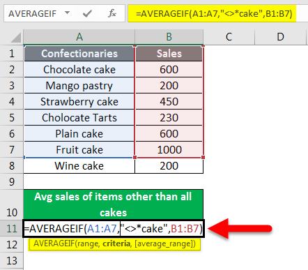
Below is a sample sales data of confectionary items. If we want to know the average sales for all cakes instead of a specific cake, we then use a wildcard(*). Like in our case, the keyword cake is preceded by other words like chocolate, fruit, plain, etc. We can overcome this limitation by using an asterisk sign before the word “cake” to fetch the cakes’ sales data.

Similarly, we can add an asterisk sign after the search keyword if some other word follows it.

So we will write the formula as below and will add * sign before our criteria. In this case, our criteria are cakes.

After pressing the Enter key, we see the result.

If any other word follows the keyword criteria, just add an asterisk sign after the keyword /criteria. Like “cake*.”

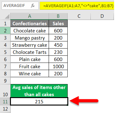
Likewise, if you want to average the sales of all other items apart from cakes, you can use the below formula using a wildcard. Which is “<>*cake”.

Press the Enter key to get the result.

AVERAGEIF in Excel – Example #5

AVERAGEIF using logical operations or numeric criteria

Many a time, we have to average cells based on logical statements like “>100” or “<100”. Or as per numeric criteria. How will we do this?

We will understand this with the help of an example.

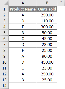
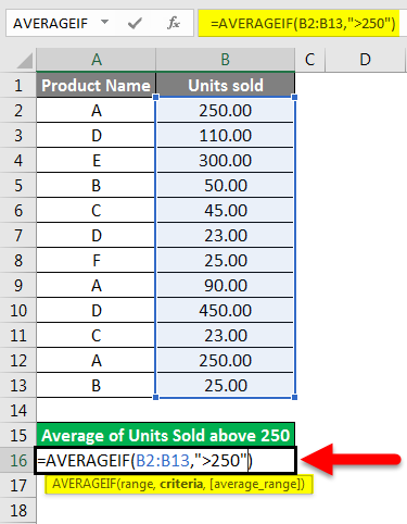
Taking our sample data. Suppose we want to know the average of units sold above 250. We will find this out as below:

After pressing the Enter key, we will get a result, as shown below.

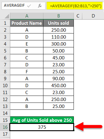
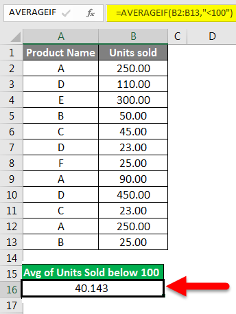
So the average of units sold above 250 belongs to products E and D. Similarly, if we want to know the average units sold below 100. We can find this, as shown below:

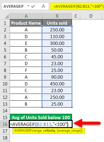
After pressing the Enter key will give us the result.

This is how we can use AVERAGEIF with logical statements as criteria.

Things to Remember

• If the criteria for calculating the average numbers are text or logical expression, they should always be written in double-quotes.
• In case no cell in the range meets the criteria for average or the range is empty, the function will return #DIV0! Error.
• If the cell as criteria is blank, the function will take it as a 0.
• Excel treats the default “criteria” operand as equals to; other operands may include >,<,<>, >=and <= as well.
• Suppose any of the cells in a range has True or False. The function will ignore it.

Recommended Articles

This has been a guide to AVERAGEIF in Excel. Here we discuss how to calculate Average using AVERAGEIF Function in Excel and practical examples, and a downloadable excel template. You can also go through our other suggested articles–

1. MAX IF Function in Excel
2. Weighted Average in Excel
3. Excel Average Formula
4. Excel AVERAGE Function