Updated August 24, 2023
Flowchart in Excel
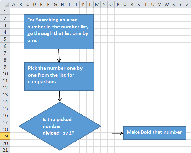
A flowchart in Excel is used to create a flow of any process from start to end. Excel flow Charts can be created by using different shapes available in the Insert menu’s Shape option.
Every flow chart starts and ends with the Rectangle, and a one-directional arrow represents the direction of the data flow. If any process or function happens, we usually show it with a Diamond shape. Every shape has a different meaning when we use them in Flow Chart. Always name each step and shape to make it more meaningful.
How to Create a Flowchart in Excel?
Excel provides the in-built shapes or symbols through which we will do preliminary formatting and manual adjustments while creating a flowchart in Excel.
It includes the below steps for creation.
Format a Grid
Although this step is an option, it will help us create uniform shapes if you follow this step. We change the column width for all the columns to equal the default row height, which helps us create more uniform shapes.
For this, follow the below steps:
Step 1 – Select all the cells in the spreadsheet by clicking on the box in the extreme upper left corner.
Step 2 – Right-click on any column heading, and it will open a drop-down list of items. Click on Column Width.
Step 3 – By default, it’s showing 8.43. Change this to 2.14, which is equal to 20 pixels. Click on OK.
Enable Span
This process helps to resize shapes and is easy to place on the grid.
For this, follow the below steps:
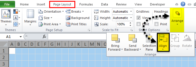
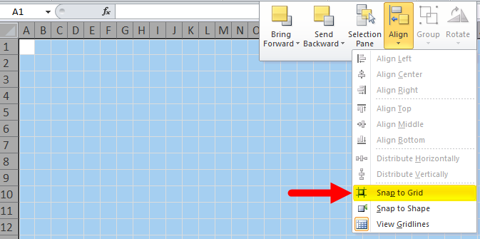
Step 1 – Go to the Page Layout tab. Click on Align option under Arrange section, as shown in the below screenshot.
Step 2 – It will open a drop-down list. Click on the Snap to Grid option from the list.
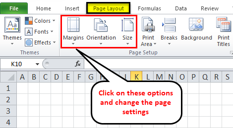
Set the Page Layout Setting
It is required to set up the page layout for a flowchart so that you know your boundaries before creating the flowchart in Excel.
Click on the page layout tab and set the Margins, Orientation, and Size options under Page Setup to change the settings. Then, refer to the below screenshot.
Add Shapes to Flowchart in Excel
Follow the below steps to add the first shape to your Excel flowchart:
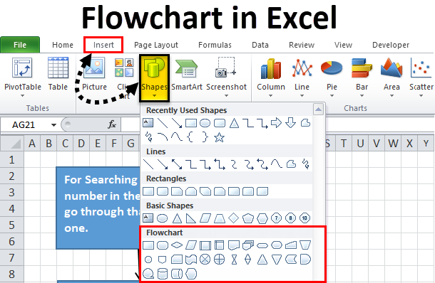
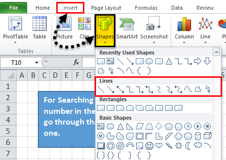
Step 1 – Go to the INSERT tab. Click on the Shapes option under the Illustrations section. It will open a drop-down list of various sections with different options and styles. Refer to the below screenshot.
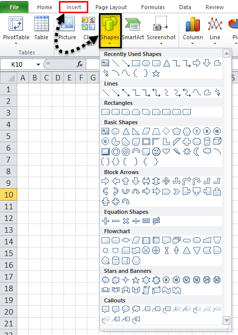
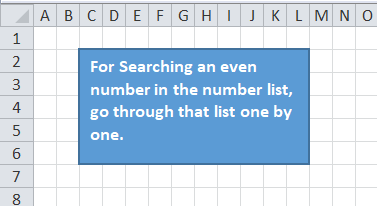
Step 2 – Click on any shape under the Flowchart section and drag it on the worksheet. We are dragging the rectangle on the worksheet, which refers to the process stage.
- As we have enabled the Snap to Grid option, this shape automatically snaps the gridlines when you draw it.
Add More Flowchart Shapes in Excel
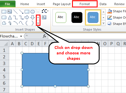
After drawing the first shape on your worksheet, an additional FORMAT tab opens, as shown in the below screenshot.
You can create more shapes using a drop-down under the Insert Shapes section.
You can write the text inside the shape after clicking inside the shape area.
Add Connector Lines Between Shapes
Once you have created multiple shapes on the worksheet, you need to add those shapes with a connecting line.
For this, follow the below steps:
Step 1 – Go to the INSERT tab and click on the Shapes option under the Illustrations section or Go to the new Format tab and click on the Insert Shapes dropdown. Choose the line which you want to use as a connector between shapes. Refer to the below screenshot.
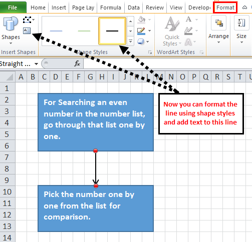
Step 2 – A plus icon will appear on the worksheet after clicking on the line symbol. Now click on the first shape you want to connect and click on the connection point from where you want the line to start. Drag that line to the next shape and release the mouse when the connector establishes well.
Step 3 – You can format the line connector and add text, as shown in the screenshot below.
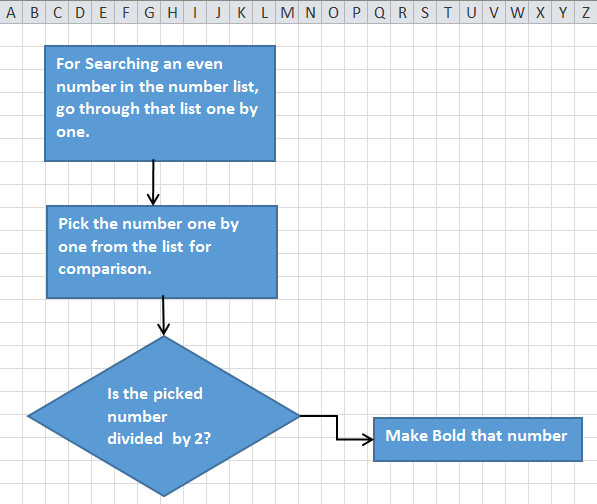
Step 4 – Now, we add more shapes with connecting lines, as shown in the below screenshot.
For Making Notes in Excel Flowchart
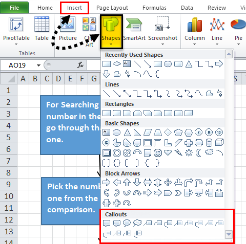
You can use Callout for making notes, and it looks different in appearance.
For this, follow the below steps:
- Go to the INSERT tab and click the Shapes option or the new FORMAT tab. Click on any shape under the Callout section, as shown in the below screenshot.
Drag the callout on the worksheet and place it in the desired position. Add text to it as we did in the above screenshot.
Formatting of Flowchart in Excel
You can format the flowchart’s shapes, connecting lines, text, etc.
Follow the below steps for this:
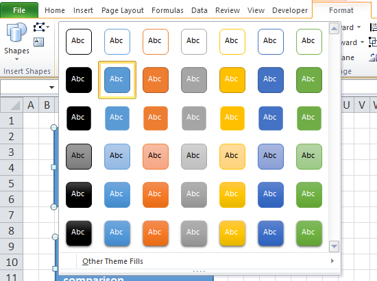
- Select all the shapes together using the SHIFT key and click on the FORMAT tab. Click on the drop-down arrow under the Shape Styles section, as shown in the below screenshot.
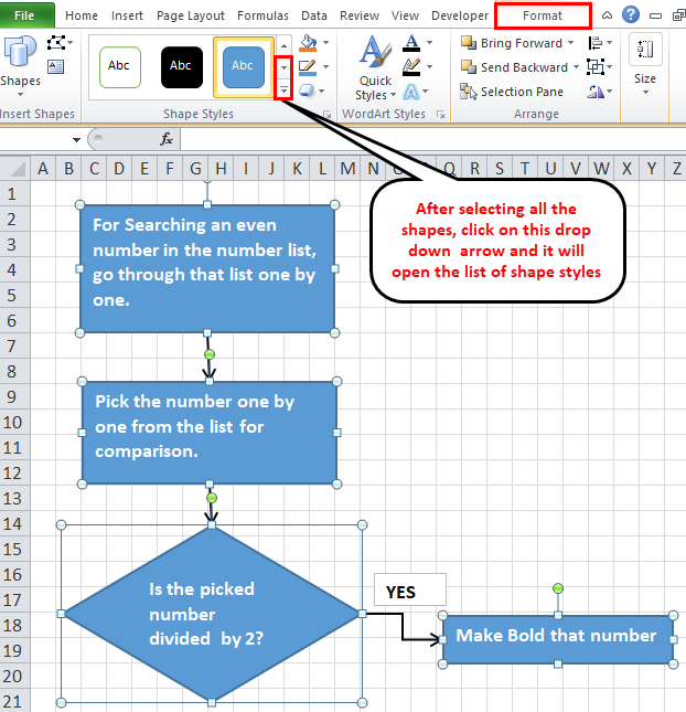
- It will open a list of various options. Choose any of them as per the requirement, and it will add the theme to the shape.
- In the same way, you can format the connecting lines and texts.
- You can align the text using Alignment and format the text by using Font under the HOME tab.
Things to Remember about Excel Flowcharts
- While choosing the Theme on the Page Layout tab and changing the Margins, Orientation, and Size will change the fonts and color themes and the height and column width, which can change the shapes available on that page.
- You can also draw a flowchart in Excel using the Smart ART option available under the Illustration section in the INSERT tab.
Recommended Articles
This has been a guide to Flowchart in Excel. Here we discuss how to create a Flowchart in Excel, practical examples, and a downloadable Excel template. You can also go through our other suggested articles to learn more –
