Updated August 21, 2023
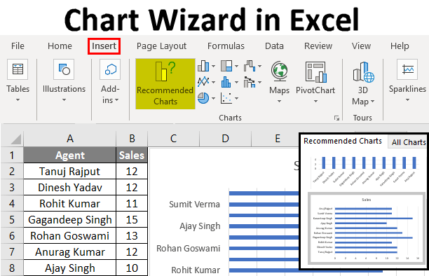
Chart Wizard in Excel
Chart Wizard in Excel is used to apply different charts, which can be Column, Bar, Pie, Areas, Line, etc. Now named Chart in the new version of MS Office, is available in the Insert menu tab. To create a chart in Excel, select data with at least one parameter that can be mapped, then from the Insert menu tab, select any chart type of choice. This will quickly create generate the Chart. We can even change the Chart’s color, add data labels, or a trend to make it more meaningful.
How to Use a Chart Wizard in Excel?
Let’s understand the working of it with the below simple steps.
Example #1 – Create a Chart using Wizard
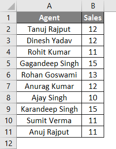
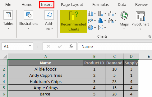
Using this Wizard, you can use any data to convert it into a chart. Let’s consider the below data table as shown in the below table and create a chart using Chart Wizard.
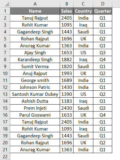
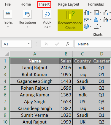
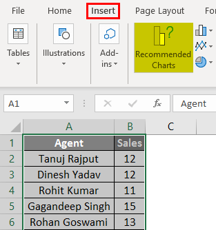
- First, select the data from which you want to create the Chart, then go to the Insert tab and select Recommended Charts Tab.
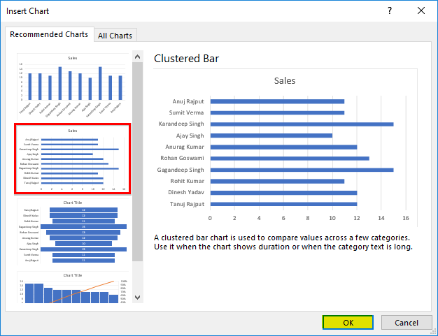
- Select the Chart and then click on OK.
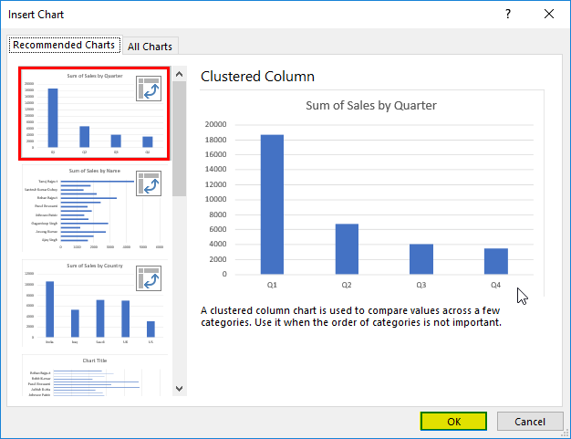
- And the output will be as shown in the below figure:
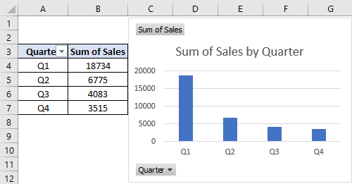
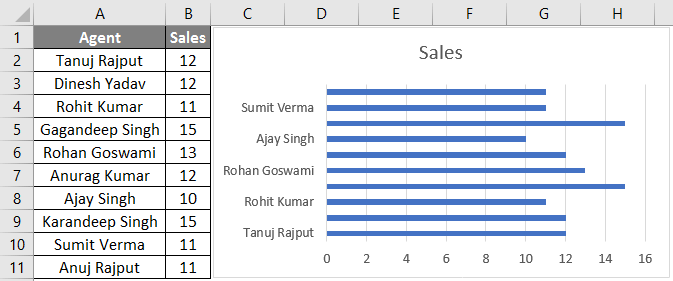
Example #2 – Create a Chart for Sales Data
Let’s consider the below data set as shown in the below table.
- Select the sales data from which you want to create the Chart, then go to the Insert tab and select Recommended Charts Tab.
- Select the Chart and then click on OK.
- And the output will be as shown in the below figure:
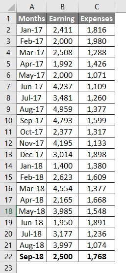
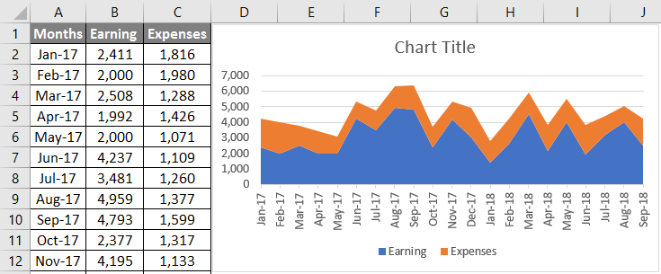
Example #3 – Create a Chart for Earning and Expenses Data
Let’s consider the below earning and expenses data set to create the Chart using chart wizard.
Here are the steps as follows:
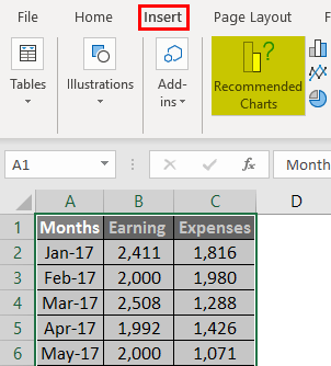
- First, select the data, then go to the Insert tab and select Recommended Chart Tab.
- Pick any chart type, and then click OK.
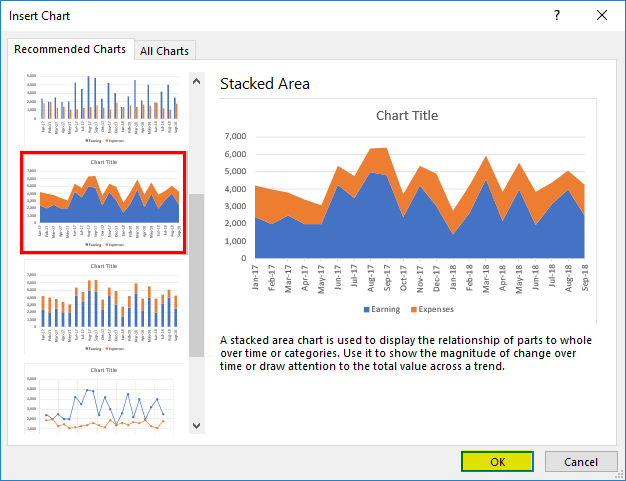
- And the output will be as shown in the below figure:
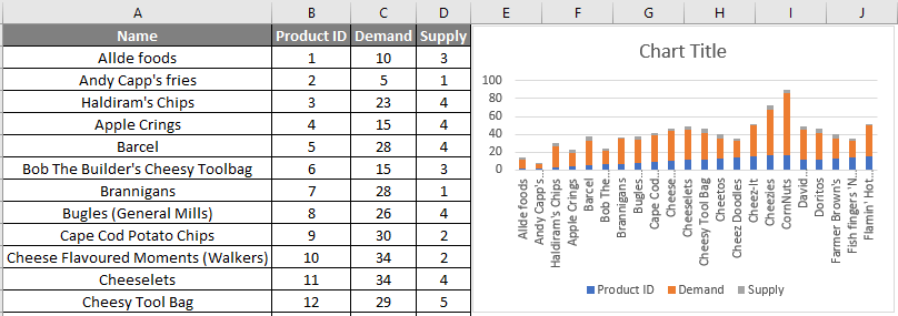
Example #4 – Create a Chart for Demand and supply Data
Let’s consider the below demand and supply data to create a chart using the chart wizard in Excel.

The steps are the same as in the previous examples; select the data below, then Go to the Insert tab and select Recommended Chart Tab.
Select the Chart which you want to create, then click OK.

And the output will be as shown in the below figure:
Things to Remember
- The Chart Wizard is simple and easy and is used to create an attractive chart using simple mouse clicks.
- The Chart wizard provides simple steps to create complex charts.
Recommended Articles
This has been a guide to Chart Wizard. Here we discussed How to use a Chart Wizard in Excel, examples, and a downloadable Excel template. You may also look at these helpful Excel articles –
