Updated May 16, 2023
Dynamic Tables in Excel (Table of Contents)
Dynamic Tables in Excel
Dynamic Table is the Table where we have to update the range of data repeatedly. The Pivot Table option can create dynamic Tables in Excel. For this, select the complete data to be included in Dynamic Table and then click on the Pivot Table option under the Insert menu tab or press the shortcut ALT + N + V simultaneously to apply it. Then drag and drop the required fields into the relevant section to create a Dynamic Table. We have to refresh the pivot table if there are any changes in the source data.
Create Dynamic Range Using Excel Tables
If you have heard of Excel tables and have not used them before, then this is the article you need the most. Excel Tables are dynamic and allow us to interpret the data once the addition and deletion happen.
We have another tool called Data Tables, which is a part of What-If-Analysis. So please don’t get confused with it.
How to Create Dynamic Tables in Excel?
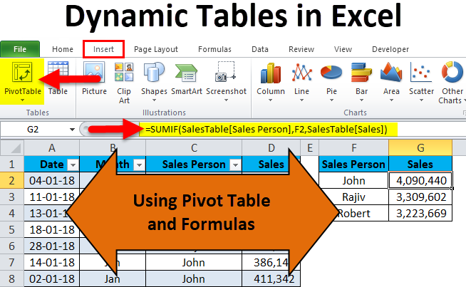
There are two basic ways to create dynamic tables in Excel – 1) Using Pivot Table and 2) Using Formulas.
Dynamic Tables in Excel – Using Pivot Table
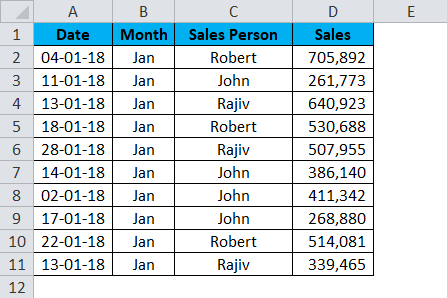
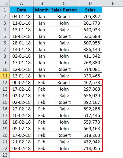
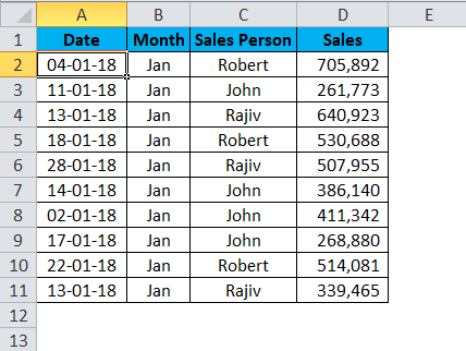
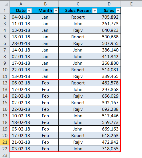
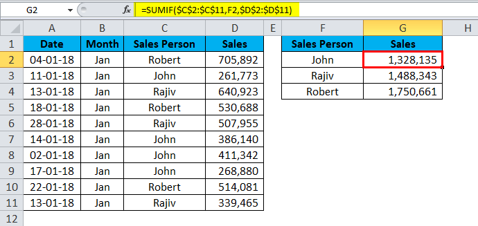
I have a sales table for the month of Jan… This sales data includes Date, Month, Sales Person, and Sales Value.
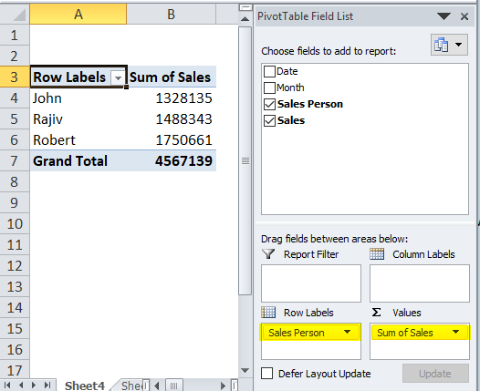
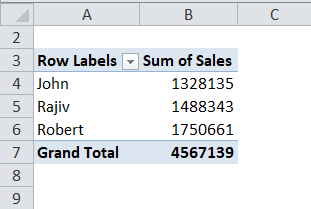
Now I want to get the total of each Sales Person by using a pivot table. Follow the below steps to apply the pivot table.
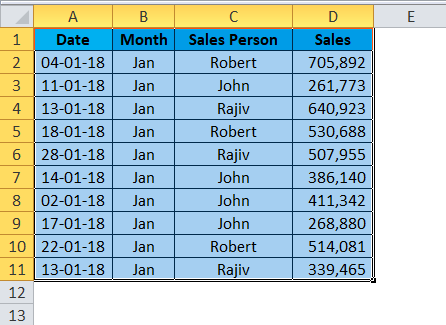
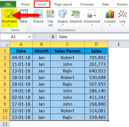
Step 1: Select the entire data.
Step 2: Select the pivot table from the Insert tab.
Step 3: Drag and drop the Sales Person heading to Rows and Sales Value to Values once the pivot is inserted.
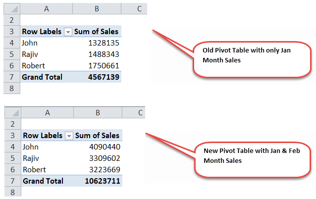
Step 4: Now I got sales updates for the month of Feb. I pasted it under Jan month sales data.
Step 5: If I refresh the pivot table, it will not give me an updated report because the data range is only limited to A1 to D11.
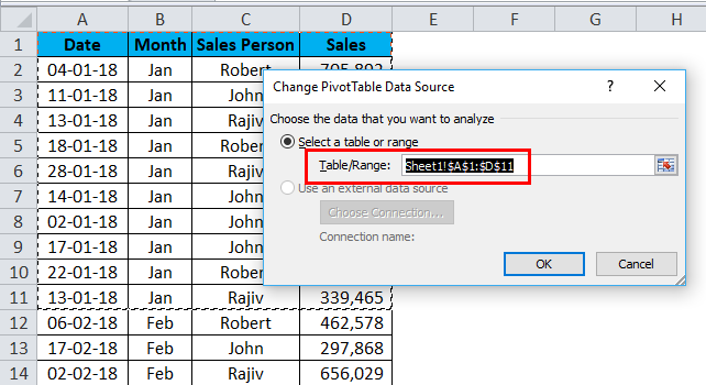
This is the problem with the normal data ranges. We must change the data source range to update our reports every time.
Create a Dynamic Table to Reduce Manual Work
By creating tables, we can make the data dynamic.
Step 1: Place the cursor anywhere in the Jan month sales data.
Step 2: Now press Ctrl + T, which is the shortcut key to insert tables. It will show you the below dialogue box. Make sure My Table has headers checkbox is ticked.
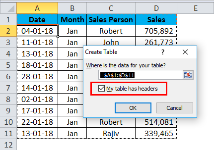
Step 3: Click the OK button; it will create a table for you.
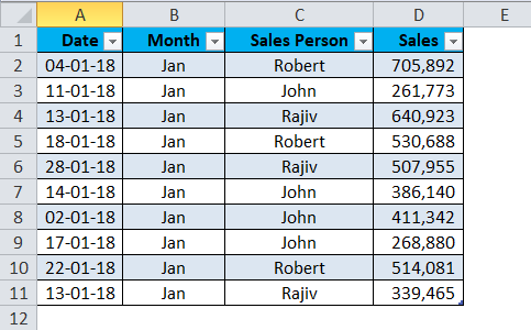
If you observe as soon as the cursor is placed anywhere in the data, it will show you the new tab in the ribbon as Design.
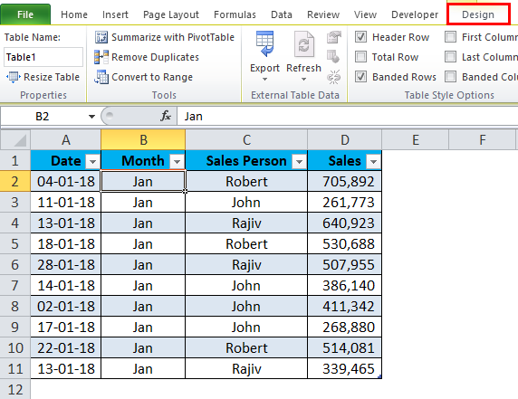
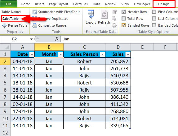
Step 4: Under the Design tab, gives a name to your Table. Give a name that is easy for you to understand.
Step 5: Now, Insert a new pivot table to this Table. (Apply previous technique) One beauty about this Table is you need not select the entire data set; instead, you can place a cursor in the Table and insert a pivot table.
Step 6: Now add Feb month sales data to this Table.
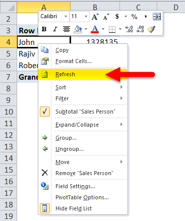
Step 7: Now go to Pivot Table and Refresh the pivot table. You can press the ALT + A + R + A shortcut key.
Step 8: It will refresh the pivot table.
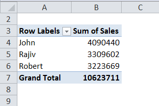
Now the pivot table shows the new values, including Feb month sales.
Dynamic Tables in Excel – Using Formulas
We can also create a pivot table with a dynamic table and apply it to formulas. Now, look at the difference between the normal and dynamic table formulas.
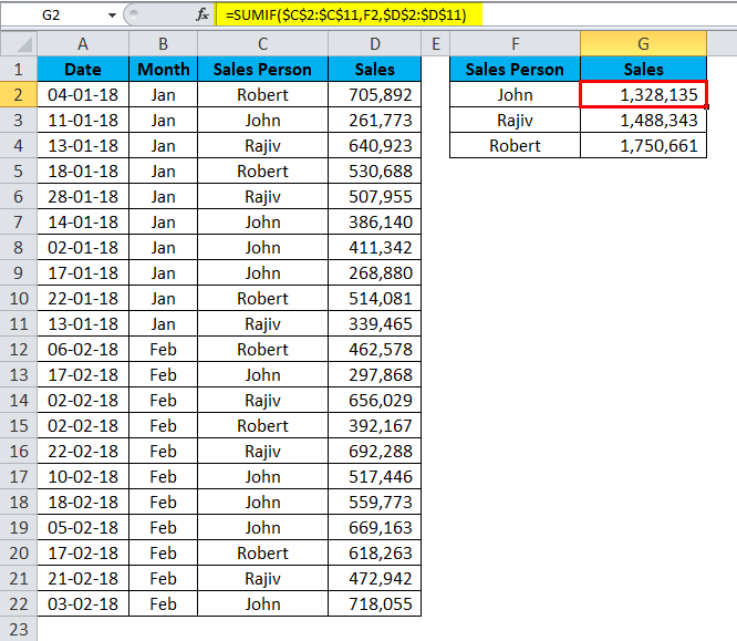
By applying the SUMIF function to the normal data range, I have received the total sales values of each salesperson.
Now I will add Feb sales data to the list.
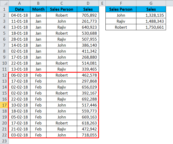
The formula still shows the old values.
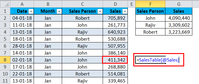
Now I will apply the formula to the Dynamic Table.
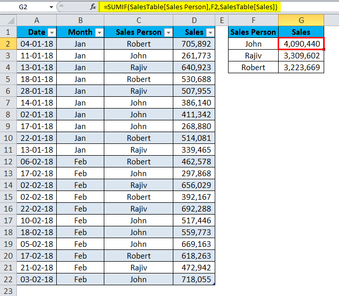
If you observe the formula, there are no ranges to the formula. It has names in it. Let me break down the formula into pieces.
=SUMIF(SalesTable[Sales Person],F2,SalesTable[Sales])
- SalesTable: This is the name of the Table.
- Sales Person: This is the column’s name we are referring to.
- F2: This is the Cell reference of Sales Person names.
- Sales: This is again the column we are referring to.
Once the Table is created, all the column headings become their references in Excel tables. Unlike in normal data ranges, we won’t see any cell ranges. These are called Named Ranges, created by the Excel Table itself.
Things to Remember About Dynamic Tables in Excel
- Ctrl + T is the shortcut key to create tables.
- All the headings refer to their respective columns.
- We use the column heading to refer to the individual cell within that column.
- We can create dynamic named ranges as well.
Recommended Articles
This has been a guide to Excel Dynamic Tables. Here we discuss how to create a dynamic table in Excel using Pivot Table and Formulas, practical examples, and a downloadable Excel template. You can also go through our other suggested articles –
