Updated August 21, 2023
Lookup Table in Excel
The lookup function is not as famous as Vlookup and Hlookup; here, we must understand that it always returns the approximate match when performing the Lookup function. So there is no true or false argument as it was in Vlookup and Hlookup functions. In this topic, we will learn about Lookup Table in Excel.
Whenever the Lookup finds an exact match in the lookup vector, it returns the corresponding value in a given cell, and when it doesn’t find an exact match, it goes back and returns the most recent possible value but from the previous row.
Whenever a larger value is available in the lookup table or lookup value, it returns the last value from the table. When we have lower than the lowest, it will return #N/A, as we have understood the same in our previous example.
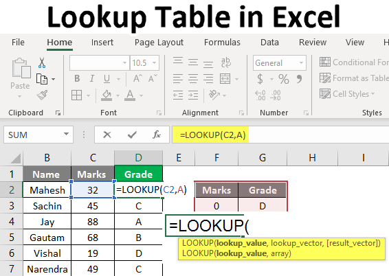
Remember the below formula for Lookup:
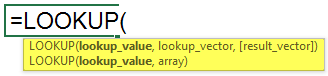
=Lookup(Lookup Value, Lookup Vector, result vector)
Here let us know the arguments:
Lookup Value: The value we are searching
Lookup Vector: Range of lookup value – (1 Row of 1 Column)
Result Vector: Must be the same size as the lookup vector; it’s optional
- It can be used in many ways, i.e., Grading students, Categorizing, retrieving approx. Position, Age group, etc.
- The lookup function assumes Lookup Vector is in ascending order.
How to Use Lookup Table in Excel?
Here we have explained how to use Lookup Table in Excel with the following examples.
Example #1
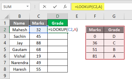
- For this example, we need data from the school students with their names and marks in a particular subject. As shown in the image below, we have the data of the students as required.
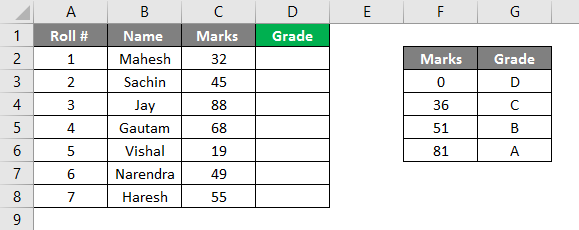
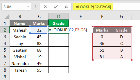
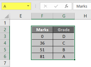
- Here also, we need a lookup vector, the value which defines marks in grades. We can see the image; on the right side of the image, we have decided the criteria for every grade; we will have to make it in ascending order because, as you all know, Look up every time assumes that the data is in ascending order. As you can see, we have entered our formula in D2 Column, =lookup(C2, F2: G6). Here C2 is the lookup value, and F2: G6 is the lookup table/lookup vector.
- We can define our lookup table by assigning it a name like any alphabet, let’s assume A, so we can write A instead if it’s range F2: G6. So as per the below image, you can see that we have given the name to our grade table as A.
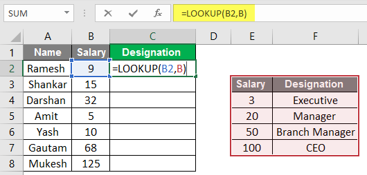
- We can place A instead of its range while applying the formula, as seen in the image below. We have applied the formula as = Lookup (C2, A), so here, C2 is our lookup value, and A is our lookup table or range of Lookup.
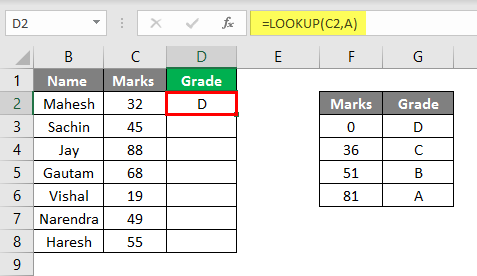
- We can see that Mahesh’s marks are 32, so from our lookup/grade table, the Lookup will look for the value 32 and 35 marks and its grade as D to show Grade’ D.’
- If we drag the same till D8, we can see all the student’s grades as per the image below.
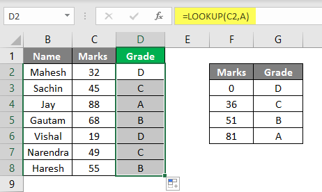
- As per the above image, you can see that we have derived the grade from the Provided Marks. Similarly, we can use this formula for other purposes; let’s see another example.
Example #2
- Like the above table, we have gathered a company’s data with the name, salary, and designations. The image below shows that we have given the name “B” to our lookup table.
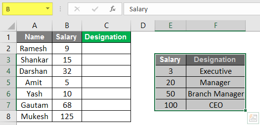
- We need the data in the designation column to put the formula in C2.
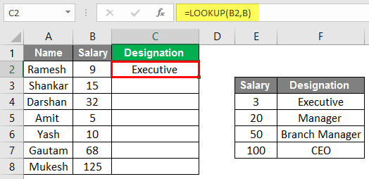
- Here we can see the Result in the Designation Column.
- Now we can see that after dragging we have fetched the designations of the staff according to their salary. We have operated this operation the same as a recent example; here, instead of marks, we have considered the salary of employees, and instead of Grades, we have considered the designation.
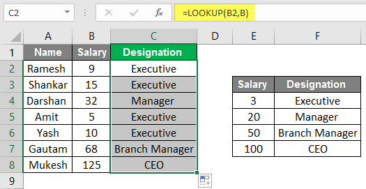
- So we can use this formula for our different purposes, academic, personal, and sometimes while making rate cards of a business model to categorize the things in manners of costly and cheap things.
Example #3
- Here as improvisation, we can make a simulator by using a lookup formula; As per the below image, we can see we have used the same data instead of the table; now, we can put data.
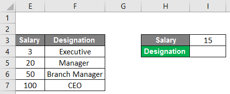
- We can see here in cell no. I4, we have applied the lookup formula, so whenever we put a value in cell no. I3, our lookup formula, will look into the data and put the appropriate designation in the cell.
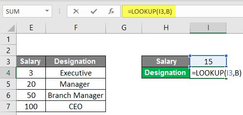
- For example, we have taken the value 15 as salary, so the formula will look up into the table and provide us with the designation according to the table, which is Executive.
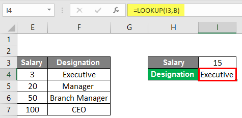
- So accordingly, we can put any value in the cell, But here is a catch, whenever we put a value higher than 100, it will show the designation as CEO, and when we put a value lower than 3, it will show #N/A.
Conclusion
The lookup function can look up values from a single column or row of the range. Lookup value always returns a value on a vector; Lookups are of two types: lookup Vector and lookup array. Lookup can be used for various purposes; as we have seen above, Lookup can be used in Grading for students; we can make age groups and various works.
Things to Remember About Lookup Table in Excel
- While using this function, we have to remember that this function assumes that the lookup table or vector is sorted in ascending order.
- And you must know that this formula is not case-sensitive.
- This formula always performs the approximate match, so true or false-like arguments will not occur with the formula.
- It can only Lookup at a one-column range.
Recommended Articles
This has been a guide to Lookup Table in Excel. We have discussed How to Use Lookup Table in Excel, Examples, and a downloadable Excel template. You may also look at these useful functions in Excel –
