Updated May 15, 2023
Introduction to Excel Table
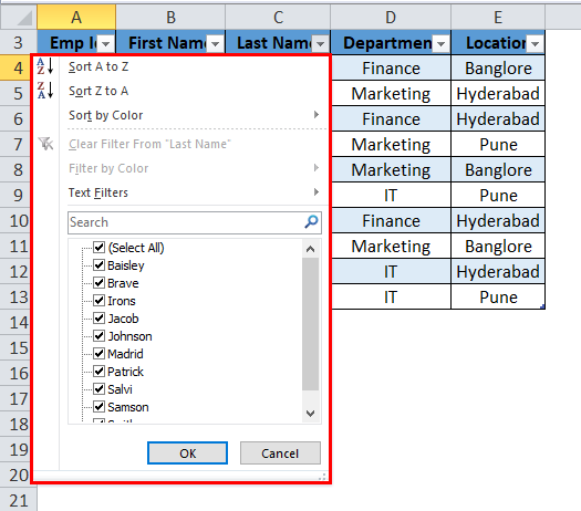
Tables in Excel are beneficial for giving structure to data sets. It has handy features from arranging the data, providing the headers, and applying filters. We can access tables from the Insert menu tab or select the shortcut key Ctrl + T. We need to select the range of cells to include and even change Table styles from the Design tab, which will appear once we select the table.
Steps need to be done before creating tables in Excel:
- First, remove all blank rows and columns from the data.
- All the column headings should have a unique name.
How to Create Tables in Excel?
It is effortless to create. Let’s understand the working of the tables with some examples.
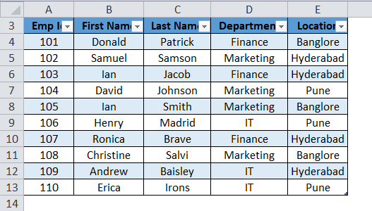
Let’s take company employee data.
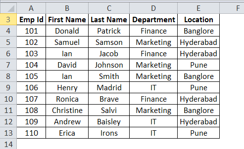
Check the data; it should not have any empty rows or columns. Put the cursor anywhere in the data and press the shortcut keys CTRL+T. It will open a dialog box.
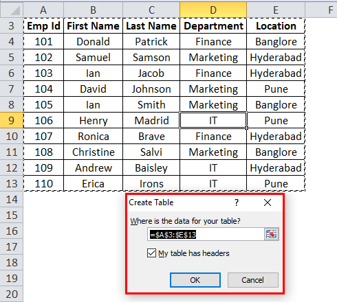
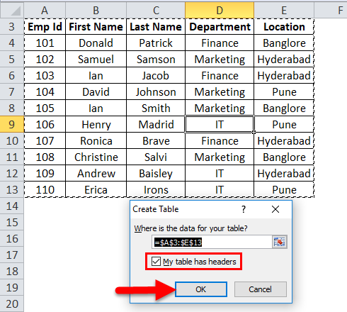
Make sure that checkbox My table has headers is ticked. It considers the first row as a header. And then click, Ok.
After clicking OK, it will create a table like the screenshot below.
As we can see, it will also open a separate Table tools design window along with the table. With the help of this, we can customize our table.
Steps for Customizing Tables in Excel
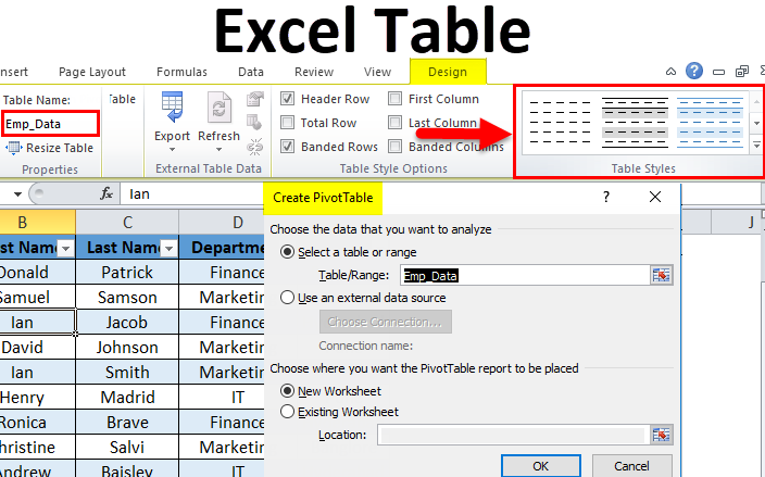
- Table Name
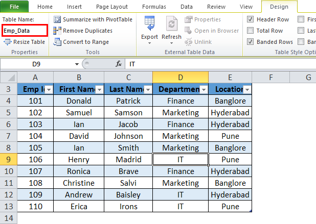
Automatically excel provides a default name. If it’s the first table, it will assign the table name as Table 1. In our example, Excel gives the table name as Table 2.
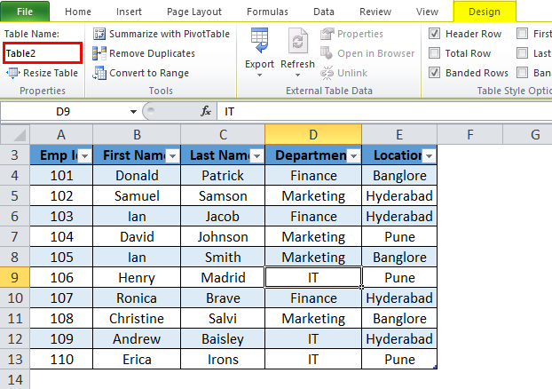
We can change this name according to the data to use it further.
Go to the Table Names field in the Design window.
Write the name of the table.
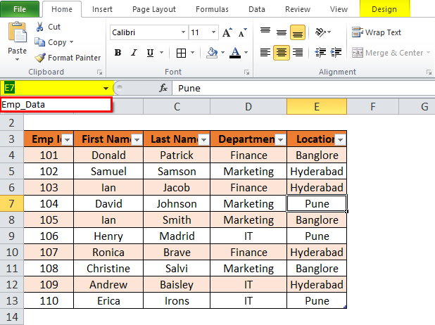
In our example, we are giving the table name as Emp_Data. Refer to the below screenshot:
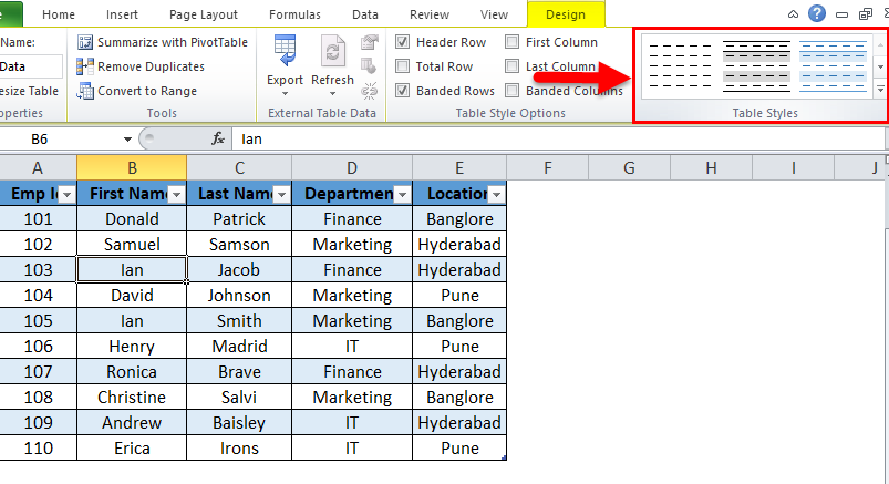
- Table Color
We can add the color to the table. Click on the Table Styles section under the Design tab and choose the color accordingly. Refer to the below screenshot:
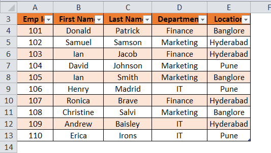
So the Output will be:
Benefits of Excel Table
- We can easily navigate between tables if we have more than one table. The Name Box drop-down shows all the table names here, and we can choose accordingly.
- When new rows or columns are added to the table, It automatically expands with the existing feature.
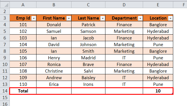
- It gives an additional feature, Total Row. The Total Row option can be easily performed SUM, COUNT, etc., operations.
For this facility, click anywhere in the table and press the shortcut key CTRL+SHIFT+T… Refer to the below screenshot:
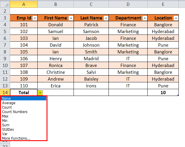
- Click on Total. It will show a drop-down list of various mathematical operations.
Note: In our example, there is no numeric data; hence it shows the total no. of records in the table.
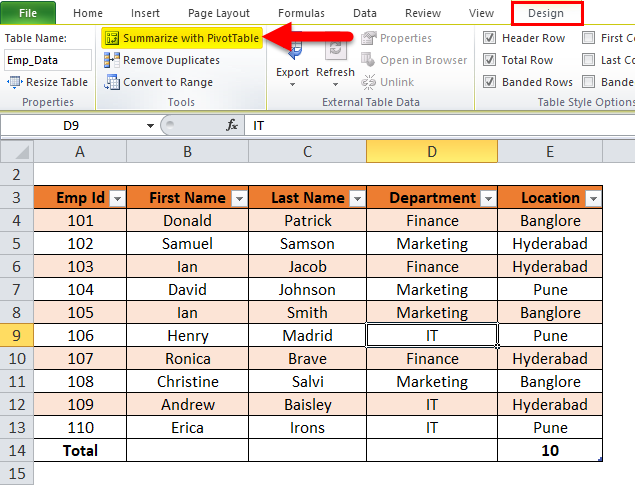
- With the help of an Excel table, we can easily create a Pivot Table. Click anywhere in the table and choose the Summarize with Pivot Table option under the Tools section. Refer to the below screenshot:
- After clicking on this, It will open a dialog box, “Create Pivot Table”.
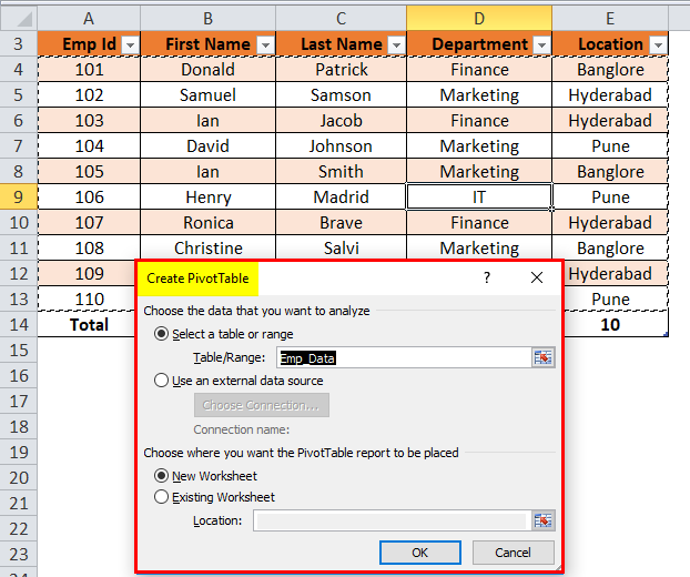
It provides all the facilities of the Pivot Table.
Things to Remember
When assigning the table name, the points below should be considered.
- The table name should not start with any special character.
- There should be no space in the table name.
- The table name can be the combination of words, but only an underscore can be used while joining the words.
- The table name should be unique if there are more than two tables.
- It should start with an alphabetic, and the maximum length should be within 255 characters.
Recommended Articles
This has been a guide to Tables in Excel. Here we discuss its uses, advantages, and how to create Excel Tables, along with an example and downloadable Excel template. You can also go through our other suggested articles –
