Updated May 15, 2023
Excel Dynamic Range (Table of Contents)
Dynamic Range in Excel
Dynamic Range in Excel allows us to use the newly updated range whenever the new set of lines is appended to the data. It just gets updated automatically when we add new cells or rows. We have used a static range where value cells are fixed, and herewith a Dynamic range; our range will change and add the data. This can be done in any function in Excel. And for this, we have an option in Excel available in the Formula tab under defined names as Name Manager.
Below are the examples for the range:
Uses of Dynamic Range
Suppose you must give an index number for a database range of 100 rows. As we have 100 rows, we need to give 100 index numbers vertically from top to bottom. Suppose we type that 100 numbers manually; it will take around 5-10 minutes. Here range helps to make this task within 5 seconds. Let’s see how it will work.
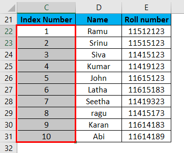
We need to achieve the index numbers shown in the screenshot below; here, I give an example only for 10 rows.
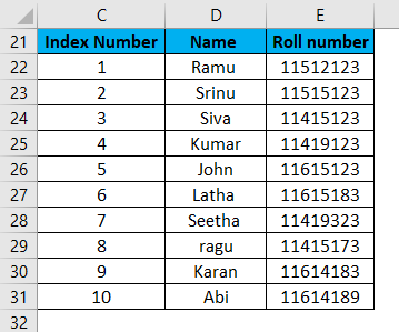
Give the first two numbers under the index number, select the range of two numbers as shown below, and click on the corner (Marked in red color).
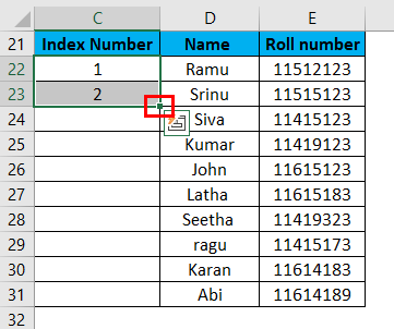
Drag until the required range. It will give the continuous series as per the first two numbers pattern.
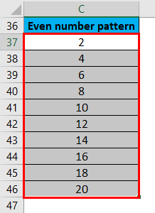
If we give the first cell 2 and the second cell 4, it will provide all the even numbers. Select the range of two numbers as shown below and click on the corner (Marked in red color).
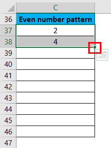
Drag until the required range. It will give the continuous series as per the first two numbers pattern.
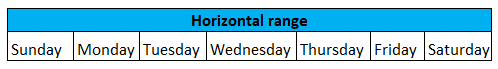
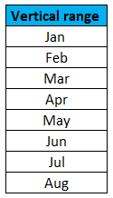
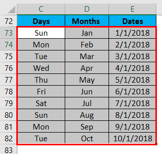
The same will apply for months, days, dates, etc.… Provide the first two values of the required pattern, highlight the range, and then click on the corner.
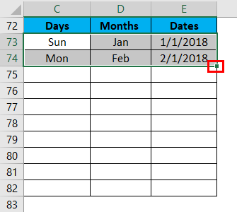
Drag until the required length. It will give the continuous series as per the first two numbers pattern.
I hope you understand what a range is; now, we will discuss the dynamic range. You can name a range of cells by simply selecting the range.
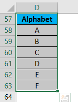
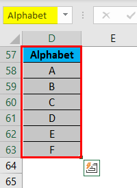
Give the name in the name box (highlighted in the screenshot).
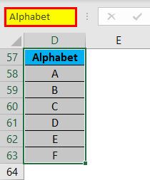
Please select the name which we added and press enter.
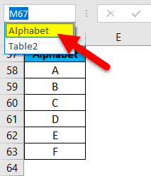
So that when you select that name, the range will pick automatically.
Dynamic Range in Excel
Dynamic range is nothing but the range that picked dynamically when additional data is added to the existing range.
Example
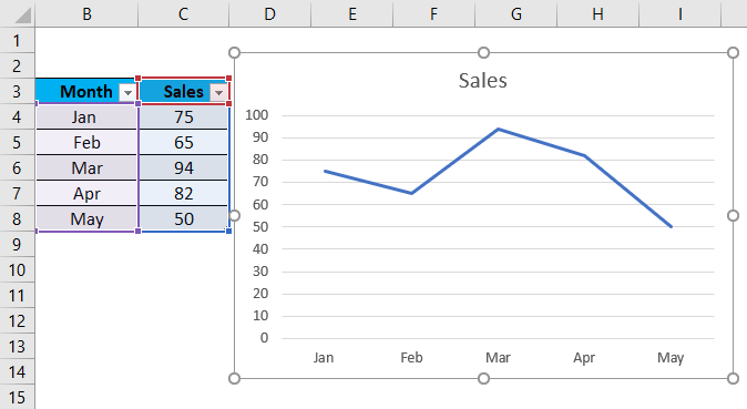
See the below sales chart of a company from Jan to Apr.
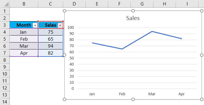
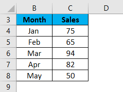
When we update May below the Apr month data’s sales in May, the sales chart will update automatically (Dynamically). This happens because we used dynamic range; hence, the chart takes the dynamic range and changes the chart accordingly.

If the range is not dynamical, then the chart will not automatically update when we update the data to the existing data range.
We can achieve the Dynamic range in two ways.
- Using the Excel table feature
- Using Offsetting entry
How to Create a Dynamic Range in Excel?
Dynamic range in Excel is straightforward and easy to correct. Let’s understand how to Create a Dynamic range with some Examples.
Dynamic Range in Excel Example #1 – Excel Table feature
We can achieve the Dynamic range by using this feature, but this will apply if we use the Excel version of 2017 and the versions released after 2017.
Let’s see how to create now. Take a database range like the one below.
Select the entire data range and click on the insert button at the top menu bar marked in red color.
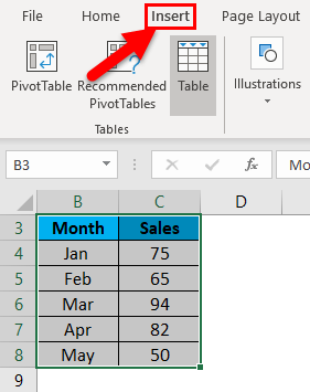
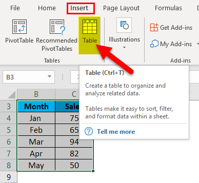
Later click on the table below the insert menu.
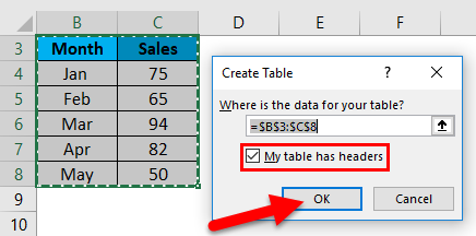
The below-shown pop-up will come; check the field ‘My table has header’ as our selected data table range has a header and Click ‘Ok.’
Then the data format will change to table format; you can observe the color also.

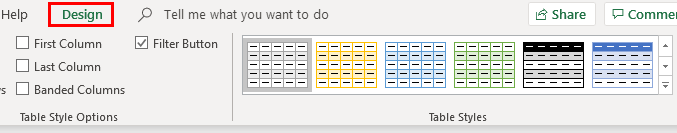
If you want to change the format(color), select the table and click on the top menu bar’s design button. You can choose the required formats from the ‘table styles.’
Now the data range is in table format; hence, whenever you add new data lines, the table feature updates the data range dynamically into a table; therefore, the chart also changes dynamically. Below is the screenshot for reference.
Click on Insert and go to charts and Click on Line chart as shown below.
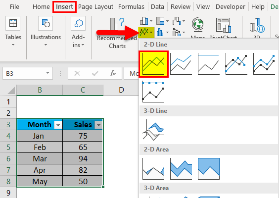
A-Line Chart is added, as shown below.
If you add one more data to the table, i.e., Jun and sales as 100, then the chart is automatically updated.

This is one way of creating a dynamical data range.
Dynamic Range in Excel Example #2 – Using the offsetting entry
The offsetting formula helps to start with a reference point and can offset down with the required number of rows and right or left with the required number of columns into our table range.
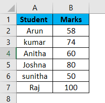
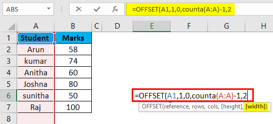
Let’s see how to achieve dynamic range using the offsetting formula. Below is the data sample of the student table for creating a dynamic range.
To explain the offset format, I am giving the formula in the normal sheet instead of applying it in the “Define name.”
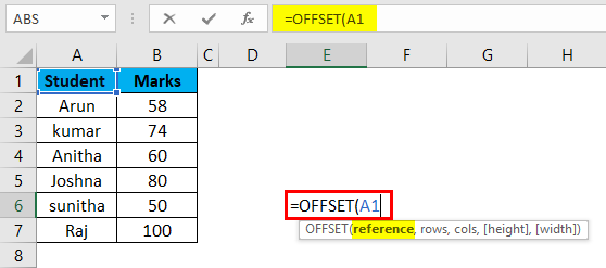
Offset entry format
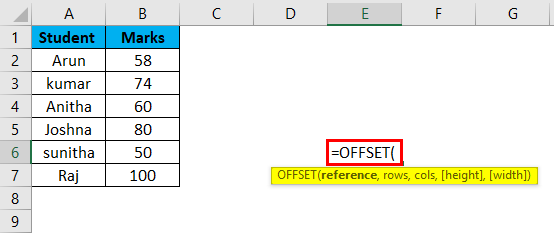
- Reference: Refers to the reference cell of the table range, which is the starting point.
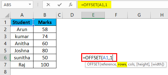
- Rows: Refers to the required number of rows to offset below the starting reference point.
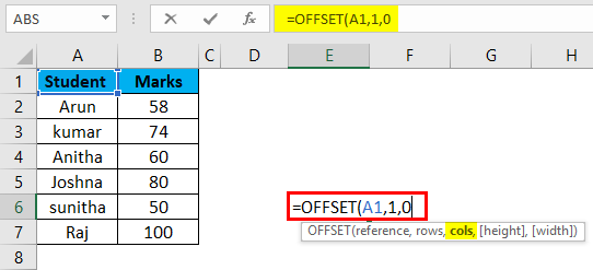
- Cols: Refers to the required number of columns to offset right or left to the starting point.
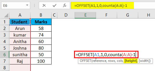
- Height: Refers to the height of the rows.
- Width: Refers to the Width of the columns.
Start with the reference cell, where a student is the reference cell where you want to start a data range.
Now give the required number of rows to go down to consider into the range. Here ‘1’ is given because it is one row down from the reference cell.
Now give the columns 0 as we will not consider the columns here.
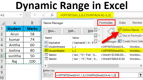
Now give the height of rows as we are not sure how many rows we will add in the future; hence, provide the ‘counta’ function of rows (select the entire ‘A’ column). But we are not treating the header into range, so reduce by 1.
Now in Width, give 2 as we have two columns here, and we do not want to add any additional columns here. If we are unaware of how many columns we will add in the future, then apply the ‘counta’ function to the entire row as we applied to height. Close the formula.
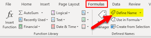
We must apply the defined name’s offset formula to create a dynamic range. Click on the “formula” menu at the top (highlighted).
Click on the option “Define Name “marked in the below screenshot.
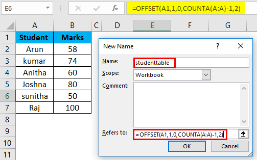
A pop-up will come, giving the name of the table range as ‘student table without space. ‘Scope’ leave it like a ‘Workbook’ and then go to ‘Refers to’ where we need to give the “OFFSET” formula. Copy the formula which we prepared priory and paste in Refers to
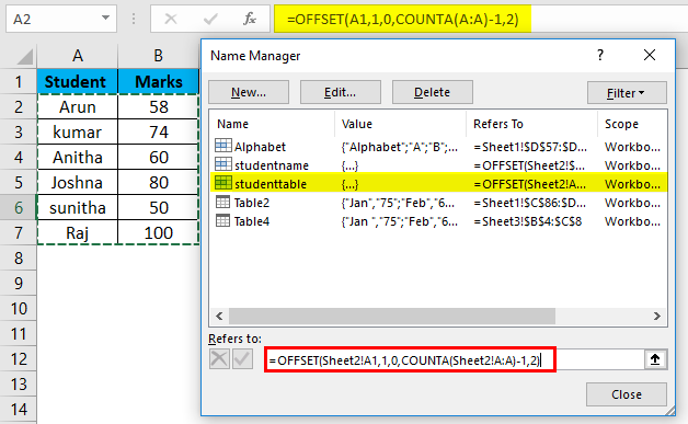
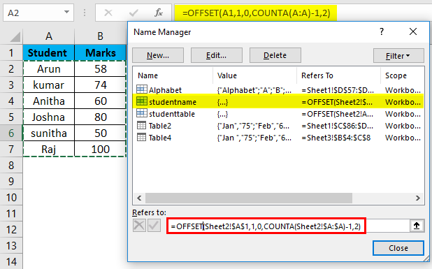
Now we can check the range by clicking on the Name Manager and selecting the name you provided in the Define name.
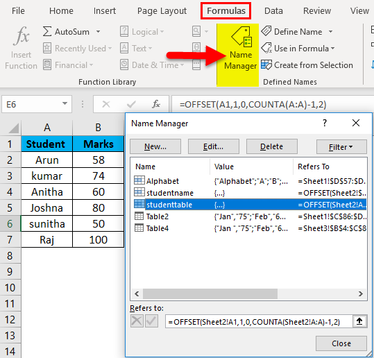
Here it is “Studenttable,” then click on the formula to automatically highlight the table range, as you can observe in the screenshot.
If we add another line item to the existing range, the range will pick automatically. You can check by adding a line item and checking the range; below is the example screenshot.
I hope you understand how to work with the Dynamic range.
Advantages of Dynamic Range in Excel
- Instant updating of Charts, Pivots, etc…
- No need for manual updating of formulas.
Disadvantages of Dynamic Range in Excel
- When working with a centralized database with multiple users, update the correct data as the range picks automatically.
Things to Remember About Dynamic Range in Excel
- Dynamic range is used when needing updating of data dynamically.
- Excel table feature and OFFSET formula help to achieve dynamic range.
Recommended Articles
This has been a guide to Dynamic Range in Excel. Here we discuss the Meaning of Range and how to Create a Dynamic Range in Excel with examples and downloadable Excel templates. You may also look at these useful functions in Excel –
