Drop Down List in Excel

What is Drop Down List in Excel?

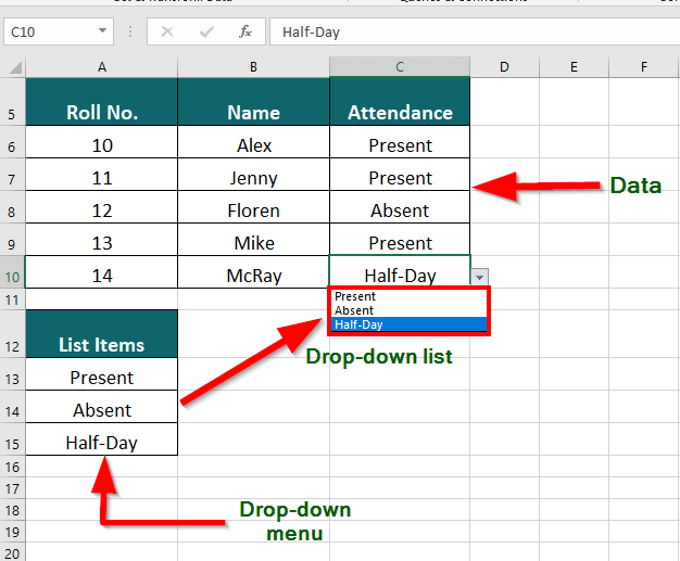
A drop-down list in Excel is a feature that allows you to choose an option from a list that appears when you click on a cell. It’s like a menu where you can pick what you want to eat. With a drop-down list, you can limit the options that someone can select to make sure they choose the correct information. We can use it to keep employee attendance records, perform large accounting data entry, or in financial modeling.

For example, we can use a drop-down list in Excel to mark student attendance in a class, reducing the risk of manual entry errors.

Key Highlights

• Dropdown lists in Excel involve a simple click on the drop-down arrow and offer an easy and efficient way to select the option we desire.
• This reduces the likelihood of making typos or errors that can occur with manual entry, improving the accuracy of data.
• The use of dropdown lists also helps to maintain the consistency and accuracy of data, which is especially important for tasks such as data analysis and reporting.
• Whenever we attempt an invalid entry, Excel displays an error alert message.
• It is possible to add new values to the dropdown list by simply adding them to the list items, giving users greater flexibility and ensuring that the list is always up-to-date.

How to Create Drop Down List in Excel?

#1: Using List Items

To create a drop-down list using list items, follow these steps:

1. Select the cell for which you want to create a drop-down list
2. Go to Data
3. Under the Data Tools group click on the Data Validation (icon)
4. Click on Settings
5. Choose List from the drop-down of the “Allow” section
6. Specify the source by selecting the list items (drop-down menu) in the worksheet.
7. Click OK.

Consider the below example which demonstrates the steps in detail:

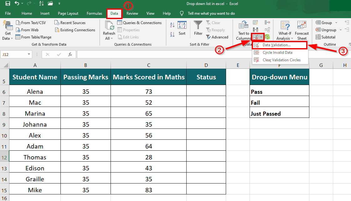
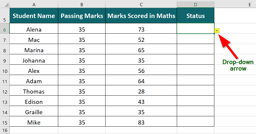
A teacher has a table of students’ Maths test marks and passing marks. They need to easily determine which students have passed, just passed, or failed. To simplify this task, the teacher wants to create a drop-down menu for selecting the appropriate result for each student.

Solution:

Step 1: Write drop-down menu options in column F

Step 2: Click on the cell where you want to insert a drop-down list and

Go To Data > under Data Tools click on the Data Validation drop-down > Data Validation

A Data Validation dialogue box will display

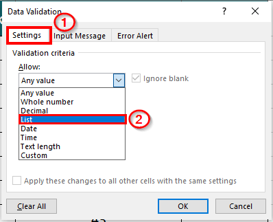
Step 3: Click on Settings > choose List from the drop-down of Allow

Step 4: Enter the Source by selecting the “Drop-down Menu” in the worksheet.

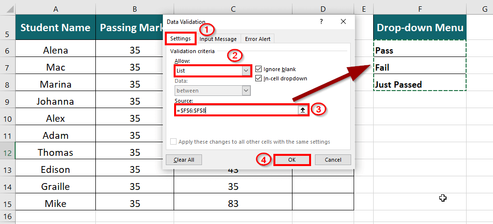
Step 5: Click OK.

This will insert a drop-down arrow adjacent to the selected cell.

Step 6: Click on the drop-down arrow to view the list items.

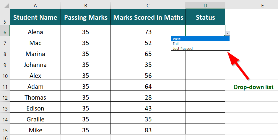
Output: The values Pass, Fail, and Just Passed are added as the drop-down list items. We can choose the desired item to fill in the cell.

Step 7: Simply drag the cross (+) to the desired row to add the drop-down list to the remaining cells.

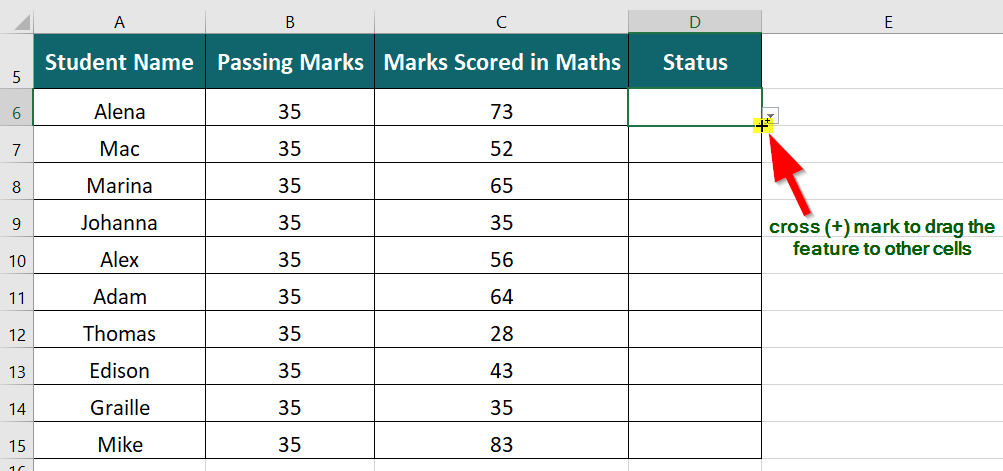
This will copy the feature and insert a drop-down list till the last cell.

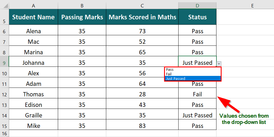
Step 8: To indicate a student’s test result based on their marks in Maths, select Pass from the drop-down list if they scored above 35 marks, select Just Passed if they scored 35 marks, and select Fail if they scored less than 35 marks.

#2: Using the Comma-Separated Values

To create a drop down list in Excel using the Comma-separated value method,  follow the given steps:

1. Select the cell for which you want to create a drop-down list
2. Go to Data
3. Under the Data Tools group click on Data Validation (icon)
4. Click on Settings
5. Choose List from the drop-down of the “Allow” section
6. Type the values that you want to add to the list
7. Click OK.

Consider the below example which demonstrates these steps in detail:

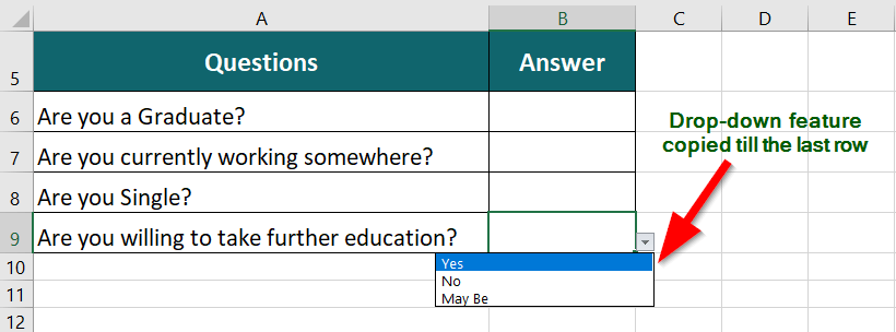
The table below shows a list of questions that candidates appearing for an interview need to answer. We want to create a drop-down list that would allow the candidates to choose from three options- Yes, No, or May Be.

Solution:

Step 1: Click on the desired cell

Step 2: Go To Data > click on the Data Validation drop-down under Data Tools group > Data Validation

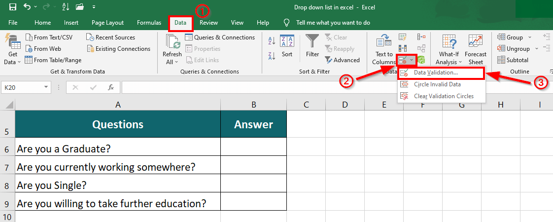
A Data Validation dialogue box will pop-up

Step 3: Click on Settings > choose List from the drop-down of Allow

Step 4: In the Source section, enter the values- Yes, No, May Be

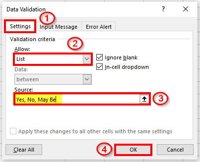
Step 5: Click OK

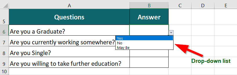
This inserts a drop-down arrow adjacent to the selected cell.

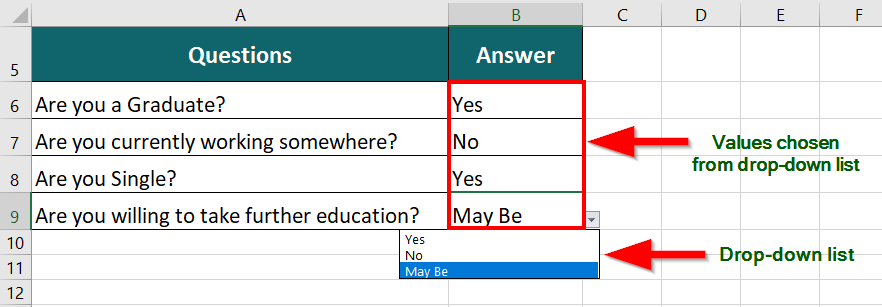
Step 6: Click on the drop-down arrow to view the list items- Yes, No, and May Be.

Step 7:  Drag the cross (+) to the last row to insert the drop-down list into the remaining cells.

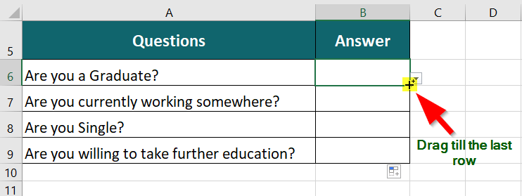
Excel adds the drop-down feature to all the rows.

Step 8: To fill the data table choose the appropriate answer from the drop-down list.

#3: Creating Dependent Drop-down List

To create a dependent drop-down list, follow the steps:

1. Select the cell that contains for which you want to create the main drop-down list
2. Go to Data
3. Under the Data Tools group click on Data Validation (icon)
4. Click on Settings
5. Choose List from the drop-down of the “Allow” section
6. Specify the source by selecting the list items (drop-down menu) in the worksheet.
7. Click OK.
8. Select the cell where you want to create a dependent drop-down list
9. Go to Data
10. Under the Data Tools group click on Data Validation (icon)
11. Click on Settings
12. Choose List from the drop-down of the “Allow” section
13. Under the Source section type the formula, =INDIRECT(cell containing main drop-down list)
14. Click OK.

The below example demonstrates the above steps in detail:

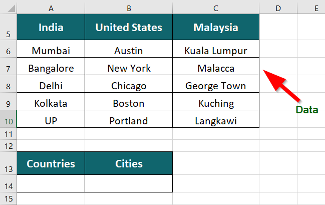
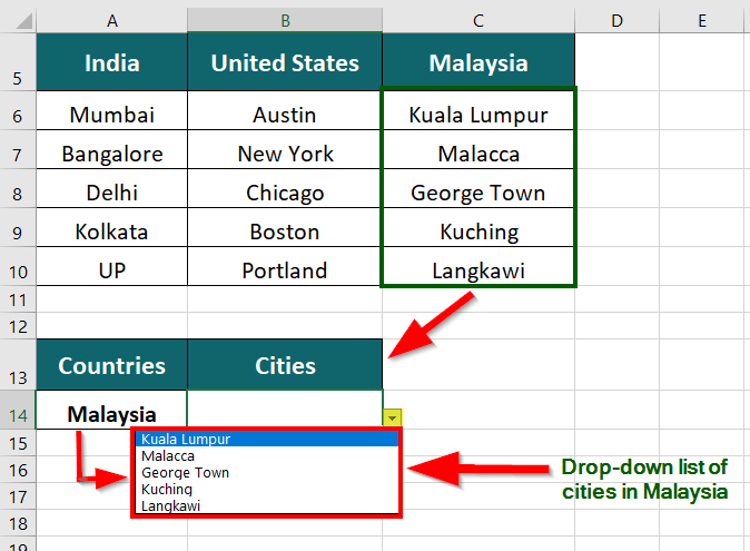
The table below mentions 3 countries- India, the United States, and Malaysia along with their popular cities. We want to create a drop down list so that whenever a user chooses a specific country it displays the respective cities in the list.

Solution:

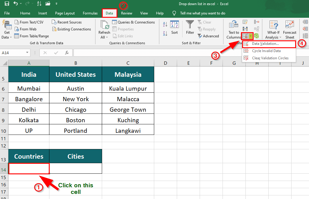
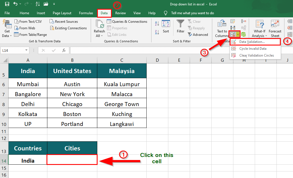
Step 1: Click on cell C14 to create a drop-down list of the countries- India, the United States, and Malaysia

Step 2: In the Excel, ribbon go to Data > under Data Tools group click on Data Validation (icon) > Data Validation

A Data Validation dialogue box appears on the screen.

Step 3: Click on Settings > choose List from the drop-down of Allow and specify the Source by selecting the countries (row 5) in the  worksheet

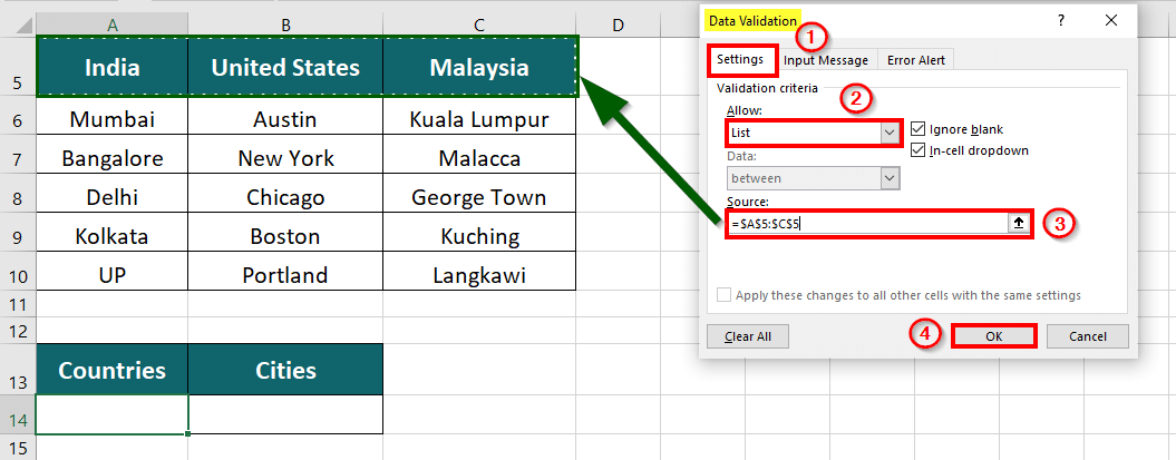
Step 4: Click OK.

Step 5: This will create a drop-down list of the country names

Step 6: To create a dependent drop-down list of cities select the cell B14

Step 7: Go To Data > under Data Tools click on Data Validation drop-down > Data Validation

A Data Validation dialogue box will appear

Step 8: Click on Settings > choose List from the drop-down of Allow

Step 9: To specify the Source enter the formula,

=INDIRECT($A$14) and click OK.

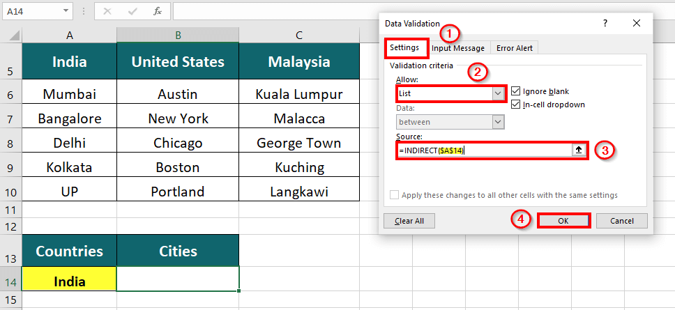
Explanation: Here, we want the drop-down list(of cities) to change as per the country. It means the drop-down list will depend upon another drop-down list, therefore, it is known as a dependent drop-down list.

So, to insert a dependent drop-down list we use the function INDIRECT followed by the cell with country names in closed brackets.

Output: A dynamic drop-down list of cities is added in cell B14.

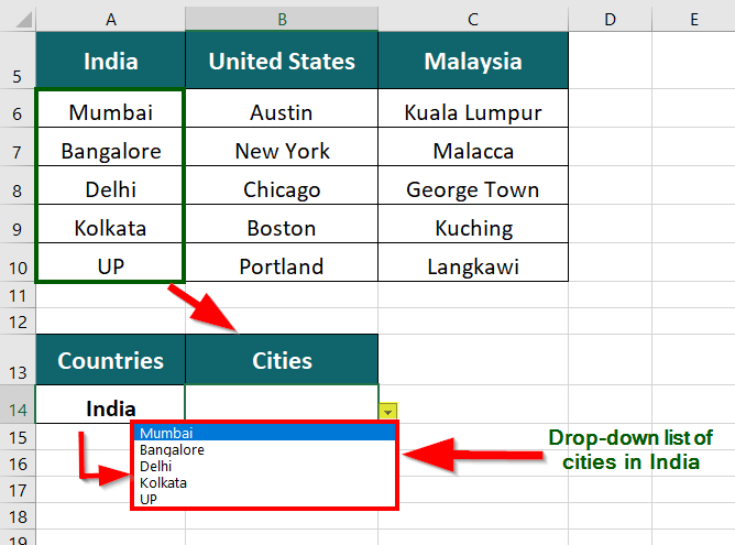
Each time you choose a different country the dependent drop-down displays a list of cities belonging to that country.

Things to Remember

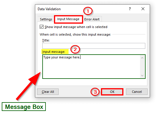
• While creating a drop-down list we can add a message from the Input Message tab in the Data Validation dialogue box. It will display a message (instruction) whenever a user clicks on the cell.

• Keep the list size reasonable and consider using scroll bars or combo boxes for longer lists.
• Ensure that the data source for the drop-down list is accurate and up-to-date.
• Consider customizing your drop-down lists with sorting options, color coding, or other formatting changes.
• Keep in mind that drop-down lists may not work in all versions of Excel or with all other software programs. Therefore, test your lists for compatibility with intended users and applications.

Frequently Asked Questions (FAQs)

What is the difference between a list and a dropdown?
A list and a dropdown are tools that let you give users a set of options to choose from in Excel. But they have some differences. A list shows the options in a column or row, while a dropdown is a button that opens up a list when you click it. Also, a list can be as big as the worksheet, while a dropdown has a limited display size.

How do I add or remove items from a drop-down list in Excel?
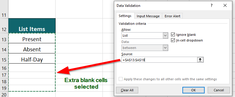
Prerequisite: While creating a drop-down list select extra blank cells while specifying the source.

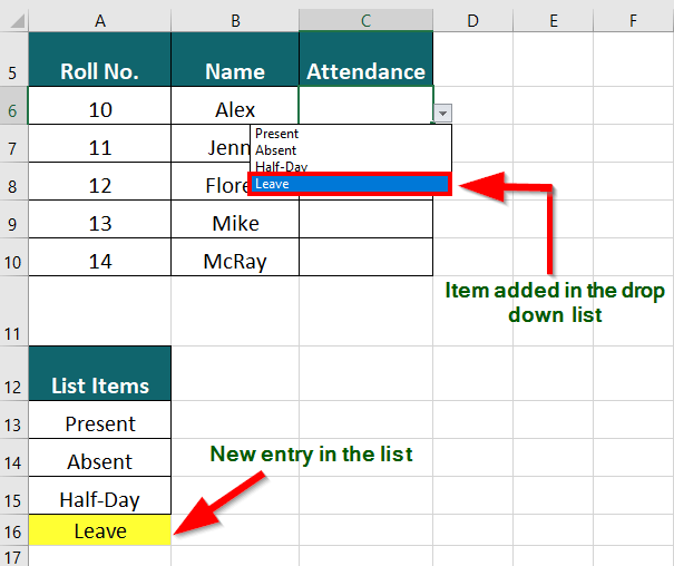
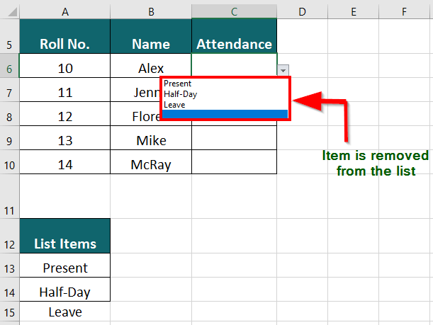
To Add an item to a drop down list enter the new value into the List Items menu. Excel will automatically insert the new value into the drop down list.

To Remove/ Delete an item from the drop down list:

Step 1: Select the entire row containing the desired value. This will shift the cells up when the value is removed.

Step 2: Right-click the selected row

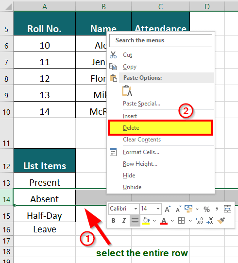
Step 3: Select Delete from the menu.

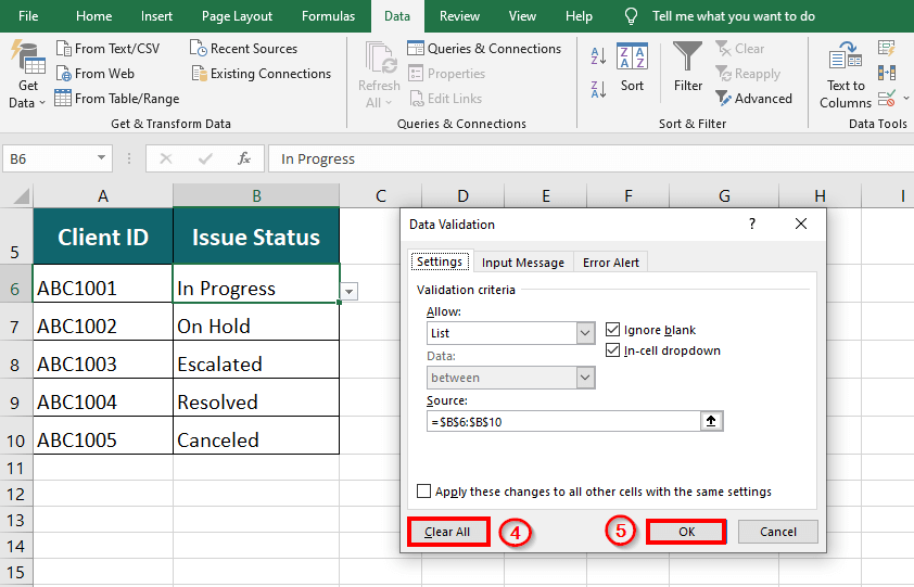
How to remove drop down list in Excel?
To remove drop down in Excel

Step 1: Select the cell from which you want to remove the drop down list

Step 2: Go to Data > Under Data Tools click on Data Validation > Clear All > OK.

What is the disadvantage of dropdown lists in Excel?
The disadvantages of a drop down list are:

• Limited space for displaying data
• Potential for data entry errors
• Limited customization options
• Compatibility issues with other software programs
• Time-consuming to set up and manage.

Recommended Articles

This has been a guide to creating a Drop down list in Excel with practical examples and downloadable excel templates. To learn about more useful features of Excel you can go through our other suggested articles-

1. Excel INDEX Function
2. Weighted Average in Excel
3. OR in Excel
4. HLOOKUP in Excel