What is Subscript in Excel?
Subscript in Excel is a formatting option that lets you display a character or a group of characters slightly below the regular text line in a smaller font size. For instance, you can display Oxygen’s chemical formula O2 as O2 by using subscript in Excel.
We often use subscripts in mathematical formulas, chemical formulas, etc. You can use them when you want to present numbers, symbols, or text in a smaller size at a lower position in comparison to the other text.
Table of Contents
- What is Subscript in Excel?
- Shortcut
- How to do Subscript in Excel? (Stepwise Examples)
- How to Add Subscript to Quick Access Toolbar?
- How to Add Subscript to Excel Ribbon?
Shortcut for Subscript in Excel
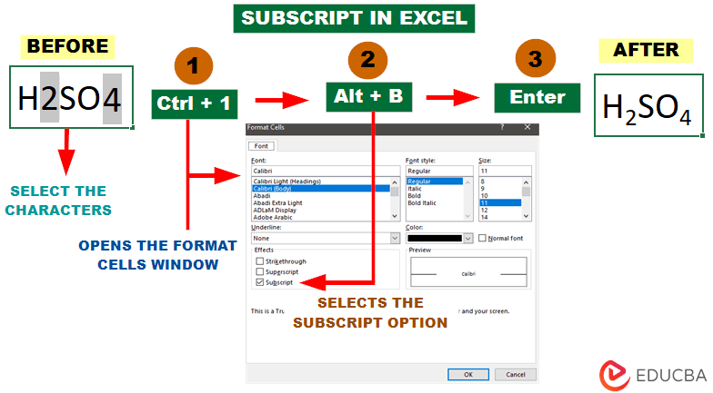
Shortcut for Windows:
- Select the character you want to format as a subscript (e.g., select 2 & 4 from H2SO4).
- Press “Ctrl + 1” to open the “Format Cells” dialog box.
- Press “Alt + B” to choose the “Subscript” option from the dialog box.
- Press “Enter” to convert the text into a subscript. As a result, the text will be H2SO4.
How to do Subscript in Excel?
Example #1: Using the Shortcut Method
Let us use subscript to change the number 2 in this sentence to subscript: “H2O is the chemical formula for water.”
1. Select the character “2” for formatting, as seen below.
![]()
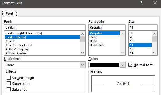
2. Press “Ctrl+1” or “Ctrl+Shift+F” to open the Format Cells dialog box.
3. Use the shortcut “Alt + B” to select ” Subscript “ in the dialog box
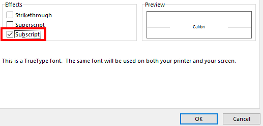
4. Confirm your choice by pressing the “Enter” This applies the formatting and closes the dialog box.
![]()
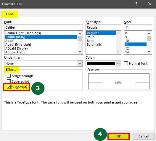
Example #2: Using the Format Text Option
Let us change “4” to subscript in the sentence: “The formula CH4 represents Methane.”
1. Select the number 4 in the cell.
2. Right-click and select “Format Cells,” and the “Format Cells” dialog box appears.
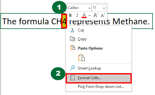
3. In the “Font” tab under the “Effects” section, checkmark the “Subscript” box.
4. Click “OK”.
Result:
The selected text or number will now appear as a subscript.
![]()
Example #3: Using Symbols
The Insert Symbol feature in Excel also helps us to insert subscripts.
Let’s say we want to add a subscript 2 to correctly complete the following sentence: “The chemical symbol for oxygen is O”.
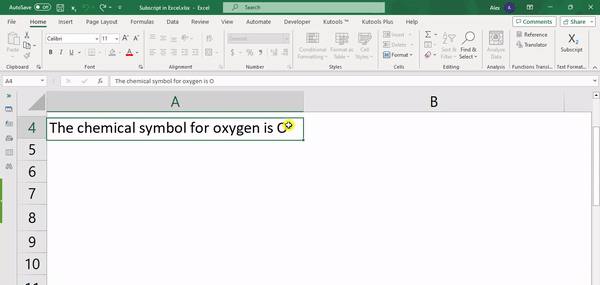
Follow the below steps to do it:
- Choose the cell and place your cursor where you want to insert the subscript
- Go to the Insert tab at the top of the Excel sheet
- Click the Symbol button in the Symbols group
- Open the Font dropdown list and select “(normal text)”
- Open the Subset dropdown list to select Superscripts and Subscripts
- Select the script character which you want to add as a subscript. For example, here, we will choose 2 as the subscript character
- Click the Insert button and close the dialog box.
Doing this will add the number as a subscript in your desired cell.
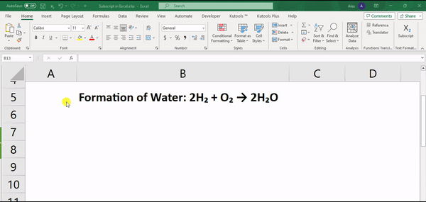
Example #4: Adding Subscript with an Equation
Excel has an equation feature that allows you to easily add equations with many subscripts or superscripts.
Let us write the equation “6CO2 + 6H2O → C6H12O6 + 6O2” using the feature.
Follow these steps to work with the Equation Editor:
- On the Excel ribbon, open the Insert
- Click on the Equation button in the Symbols (Note that you must click on the Equation button and not on the dropdown menu near it).
- In the Equation tab, click the Script button in the Structures
- Choose Subscript. Two boxes will appear.
- Use the left arrow on your keyboard to move your cursor to the larger box and type “6CO“.
- For subscript “2“, move to the smaller box using the right arrow, then type “2“.
- For regular text, move right using the right arrow and type “+“.
- Repeat steps 3-7 for your complete equation.
Example #5: Adding Subscript with Ink Equation
Follow the below steps:
- Go to Insert
- Select Equation from the Symbols
- Select Ink Equation from the Tools group in the left corner. A Math Input Control dialog box will appear.
- Select the write tool from the list and start doodling in the Write math here
- You can check the preview section to see if the equation is correct. Once done, select the Insert option to close it.
- You will see the result displayed in the box.
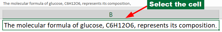
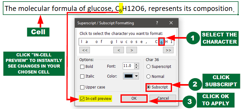
Example #6: Adding Subscript multiple characters in cells using Kutools
Imagine you have several characters in a cell that you want to make smaller and lower. Kutools for Excel has a subscript tool that can do this easily. Instead of changing each character individually, this tool lets you select the characters you want and turns them into subscripts simultaneously.
1. Click on the cell that contains the text you want to format.
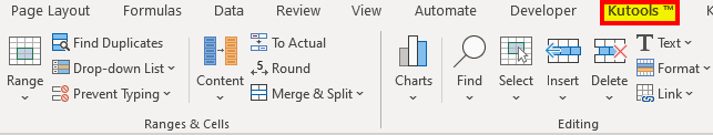
2. Go to the Excel ribbon and look for the Kutools
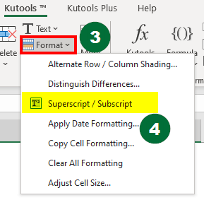
3. Under the Editing group, select the Format dropdown list
4. Click on the Superscript/Subscript option (The wording might vary based on your Kutools version).
5. A small dialog box or formatting window will open. You can use the two middle arrow buttons (< & >) or the two shift arrows (<< & >>) to view the next or previous part of the sentence.
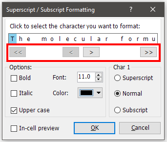
6. In the window that appears, do as follows:
-
- Select the character you want to convert to a subscript
- Select Subscript from the Char 36 You can see a preview of how your selected text looks like.
- Once you have changed all the required characters to subscript, click the OK or Apply button to confirm.
Result:
![]()
How to Add Subscript in Excel’s Quick Access Toolbar?
1. Open Microsoft Excel.
2. Find the Quick Access Toolbar near the top-left corner, above the ribbon.
3. Find the small arrow or down-facing triangle icon at the end of the Toolbar.
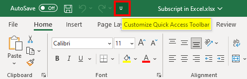
4. Click on the arrow to open a dropdown menu.
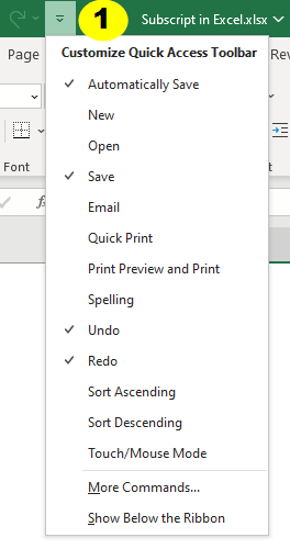
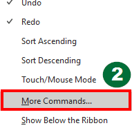
5. Select More Commands. It opens a customization window.
6. In the window, the left column lists available commands, and the right shows current quick access toolbar commands.
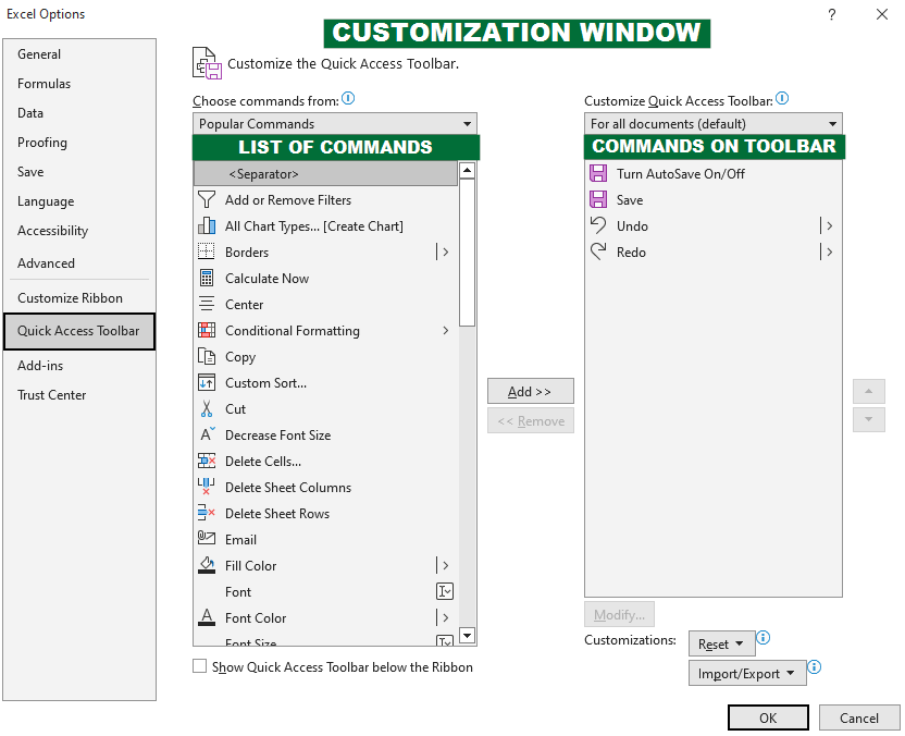
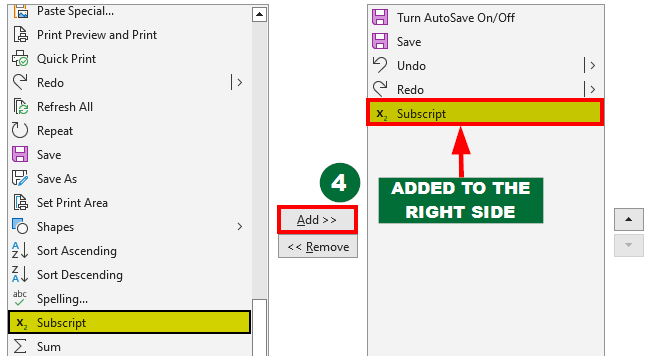
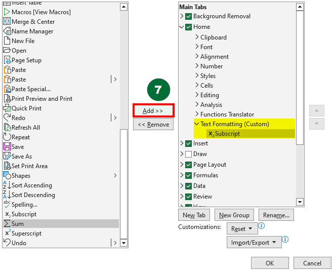
7. Find the Subscript or Format as Subscript command, and click on it to select it.
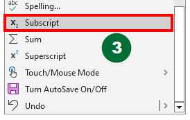
8. Click the Add button between the two columns to add the command to the Quick Access Toolbar.
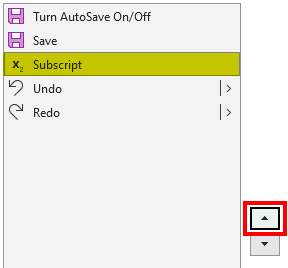
9. You can use the up and down arrows on the right side of the customization window to rearrange the commands.
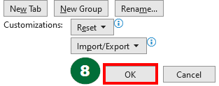
10. Once satisfied, click “OK” to close the customization window.
Result:
You should now see the subscript icon on the Quick Access Toolbar.
How to Add Subscript to Excel Ribbon?
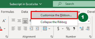
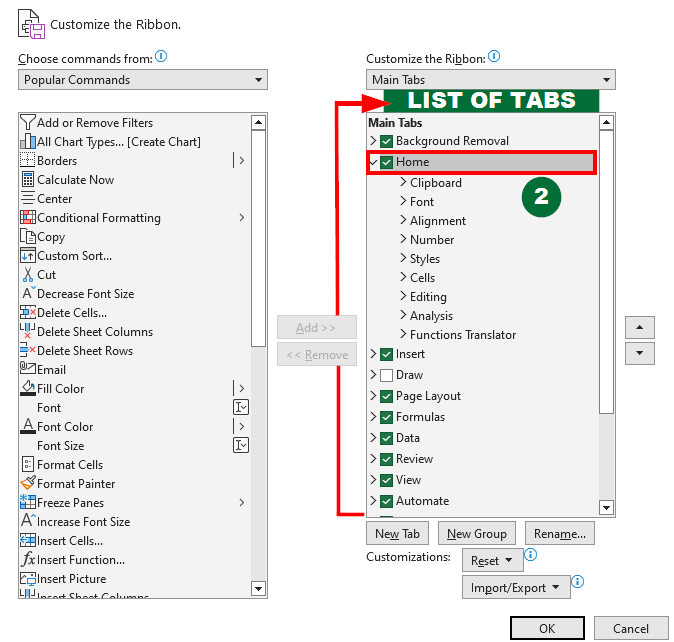
1. Right-click on the Excel ribbon (top menu) and select Customize the Ribbon from the context menu.
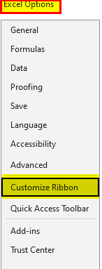
2. An Excel Options dialog box opens. Navigate to the Customize the Ribbon section on the left.
3. In the right pane, you will see a list of tabs available on the ribbon. Choose the specific tab where you want the subscript button to be.
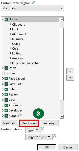
4. Click on the New Group button at the bottom.
5. Click on the Rename button and add a meaningful name.
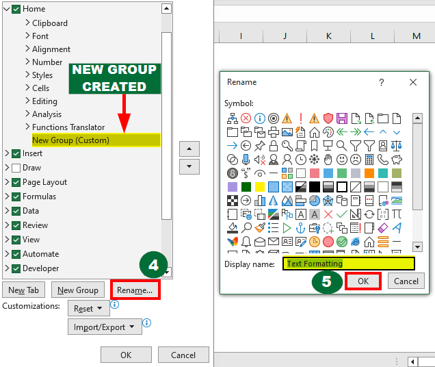
6. In the left-hand dropdown list of “Choose commands from, ” scroll down, find “Subscript,” and select it.
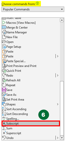
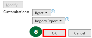
7. Click the “Add” button to move the command to the new group.
8. Click OK
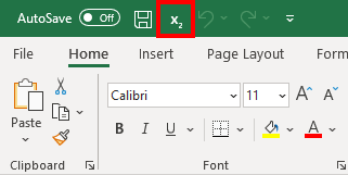
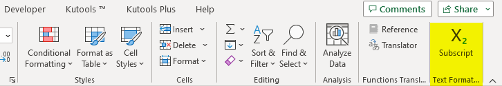
Result:
You have successfully added the subscript button to the Excel ribbon.
Frequently Asked Questions (FAQs)
Q1. Can we apply subscripts to all cell formats in Excel?
Answer: Yes, you can apply subscript formatting to any format cell in Excel, including numbers or non-textual content. Moreover, you can use subscripts for text within and for the entire cell.
Q2. What are Alt codes for subscripts in Excel?
Answer: You can use Alt codes to input subscript characters in Excel using your keyboard’s numeric keypad. For instance, the Alt code for subscript 2 is Alt + 8322. To use them, press and hold the “Alt” key, enter the Alt code, and release the “Alt” key. This will insert the corresponding subscript character at the cursor’s position.
However, remember that the availability of these characters can depend on your operating system and font settings. In that case, you can use the following formula =UNICHAR(8322). This will add subscript 2 to the cell.
Recommended Articles
This comprehensive article on Subscript in Excel shows you different ways to write and insert subscript in Excel. We have also included steps to add subscript in the quick-access toolbar and the Excel ribbon. Refer to the following articles for more Excel-related knowledge.
