Updated August 22, 2023
Shade Alternate Rows in Excel (Table of Contents)
Introduction to Shade Alternate Rows in Excel
Whenever you are working with large datasets in Excel, it is a practice that is common, and you must follow to shade the alternate rows with different colors. It makes the spreadsheet easy to read and visually appealing to the user. Showing alternate rows in a relatively small dataset is comparatively easy and can be done manually. However, manual shading will never work when you have data as large as billions and trillions of entries. In this article, we will inform you of ways to shade alternate rows with different colors in Excel.
We can usually do this task in three different ways:
- Using Excel’s Insert Table utility which automatically shades the alternate row.
- With the help of Conditional formatting without using Helper Column.
- With the help of Conditional formatting and using Helper Column.
Methods to Shade Alternate Rows in Excel
Let’s understand how to Shade Alternate Rows in Excel with some methods.
Method #1 – Shade Alternate Rows in Excel using Table Utility
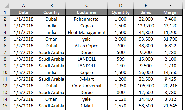
Suppose we have data of 1000 rows, as shown in the screenshot below. It is hard to shade each alternate row which consumes ample time manually. See the partial screenshot below:
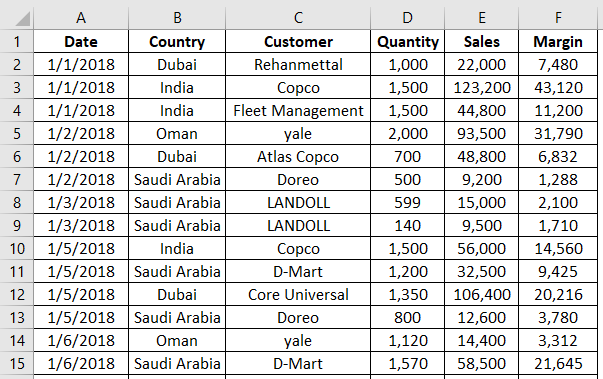
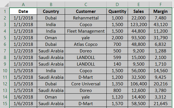
Step 1: Select all the rows where you want to shade every alternate row.
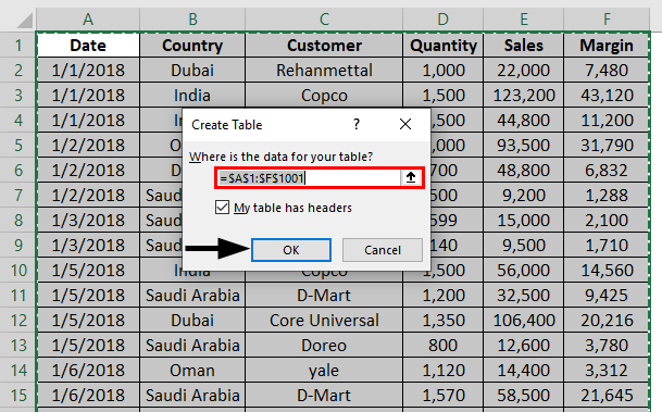
Step 2: Navigate towards the Insert tab on Excel Ribbon and click on the Table button present under Tables group. You also can do this by hitting Ctrl + T simultaneously.
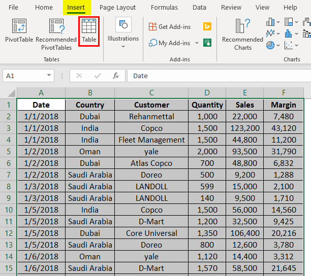
Step 3: As soon as you click the Table button, the Create Table window will pop up with the rows selection. Click the OK button to apply the table format on the selected rows.

Step 4: You also have the option to design your table in shades through the Design tab. You can navigate to more designs and create your own custom design.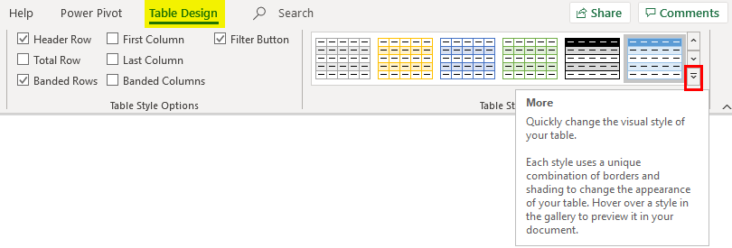
Method #2 – Conditional Formatting without Helper Column
We also can use conditional formatting to shade every alternate row in Excel. Follow the steps below:
Step 1: Highlight all non-empty rows by selecting them without a header (because we want the header color to be different, It will help recognize the headers).
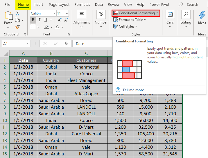
Step 2: Select the Home tab from the Excel ribbon and click the Conditional Formatting dropdown under the Styles group.
Step 3: Select New Rule… option from the Conditional Formatting dropdown.
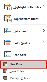
As soon as you click it, you will see a new window named New Formatting Rule popping up.
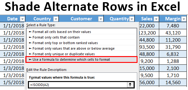
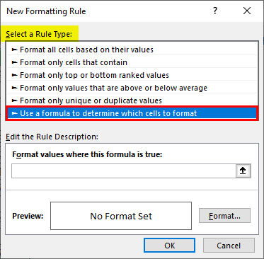
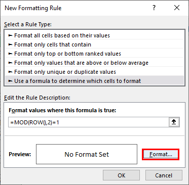
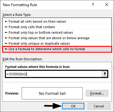
Step 4: Inside the New Formatting Rule window, select Use a Formula to determine which cell to format the rule under. Select a Rule Type: option.
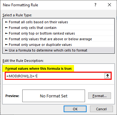
Step 5: Use formula as =MOD(ROW(),2)=1 under Formal Values, where this formula is a true box.
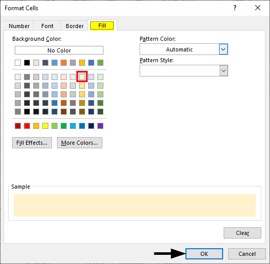
Step 6: Click the Format button to add the color shades for the alternate rows.
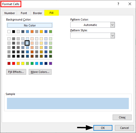
Step 7: When you press the Format button, you’ll see a Format Cells window popping up. Navigate to the Fill option and change the background color, as shown in the screenshot below. Once done, press the OK key.
You can see an output as shown below. Each cell with an Odd number is shaded through the Excel sheet.
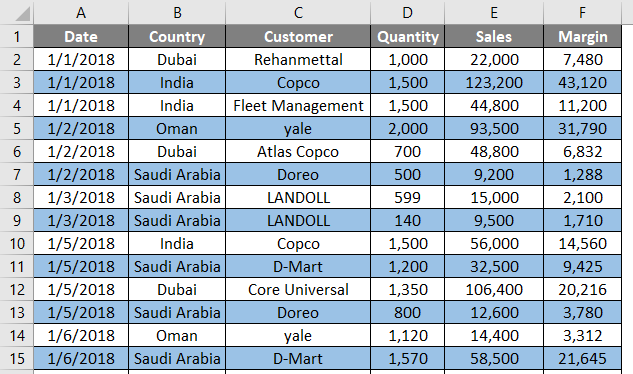
MOD() is a modulo function that can be used to find the modulus of a reminder when one number is divided by the other. For example, if we use MOD(3, 2), it means dividing the number 3 by the number 2 will give a reminder as 1. The ROW() function gives the row number for each cell the formula runs on. The combination MOD(ROW(),2) = 1 checks only those rows where a reminder is equaled to 1 (meaning odd cells). Therefore, you can see all the odd rows are shaded.
Similarly, you can shade all even rows. All you need to do is, tweak the formula as MOD(ROW(),2) = 0. This means all the rows are divisible by 2 (in other words, all even rows will be selected and shaded).
Method #3 – Conditional Formatting with Helper Column
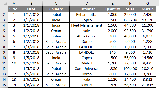
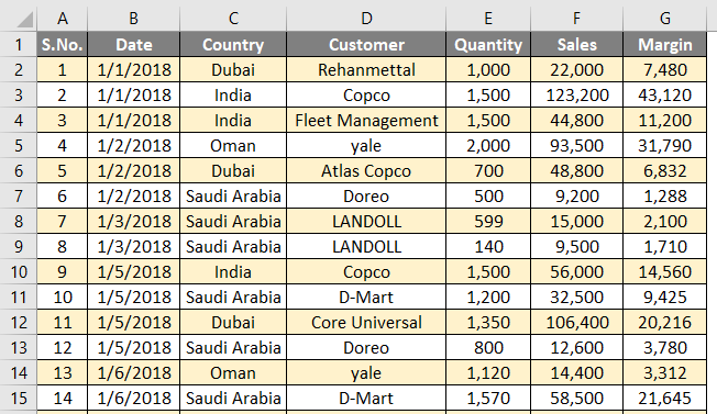
Step 1: Insert a helper column named S.NO. In the table and add the serial numbers for each row in it.
Follow the steps as same from Step 1 to Step 4 as we used in the previous example.
Step 2: Use the formula as =ISODD(A2) under Formal Values, where this formula is a true box. This formula works similarly; the previous one works in Example 1. It captures whether the value in cell A2 is odd or not. If it is odd, it performs the operation we perform on that cell.
Step 3: Again, do the same procedure as in the previous example. Click the Format button and select the appropriate color as a shade under the Fill section. Once done, press the OK button.
You can see an output as shown in the screenshot below.
These are the three easy methods to shade the alternate rows in Excel. Let’s wrap things up with some points to be remembered.
Things to Remember About Shade Alternate Rows in Excel
- The easiest way to shade every alternate row in Excel is by using the Insert Table option. It is simple, versatile, time-saving, and has different designs that give you different layouts.
- It is also possible to shade every 3rd, every 4th, or so row. All you need to do is change the divisor from 2 to the respective number (3, 4, etc.) under the MOD formula, which we use to define the row selection and formatting logic.
- ISODD and ISEVEN functions can also be used. ISODD shades all the odd-numbered rows, and ISEVEN shades all the even-numbered rows.
- You also can shade even and odd cells with different colors. For that, you need to apply two conditional formatting.
Recommended Articles
This is a guide to Shade Alternate Rows in Excel. Here we discuss the Methods to Shade Alternate Rows in Excel and the downloadable Excel template. You can also go through our other suggested articles –
