Updated August 22, 2023
Introduction to Excel Alternate Row Color
The most organization”needs to present th”ir data professionally. Applying alternate and unique colors to the data makes the sheets more perfect, making the data view colorful. In Microsoft Excel, “Alternate Row Color” is mostly used in a table to display data more accurately. In Microsoft Excel, we can either manually apply color to the rows or simply format the row to apply color shading to the specific rows and columns.
How to Add Alternate Row Color in Excel?
Add Alternate Row Colors in Excel is very simple and easy. Let’s understand how to add Alternate Row Colors with some examples.
In ExLet’swe can manually apply color to the rows by selecting a unique color. Selecting an “altern” color makes it difficult for the users. To overcome these things excel has given us a formatting table option to select a wide range of alternate row colors. Let’s look at a few examples.
Example #1 – Formatting Row Table
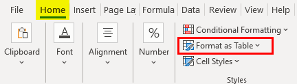
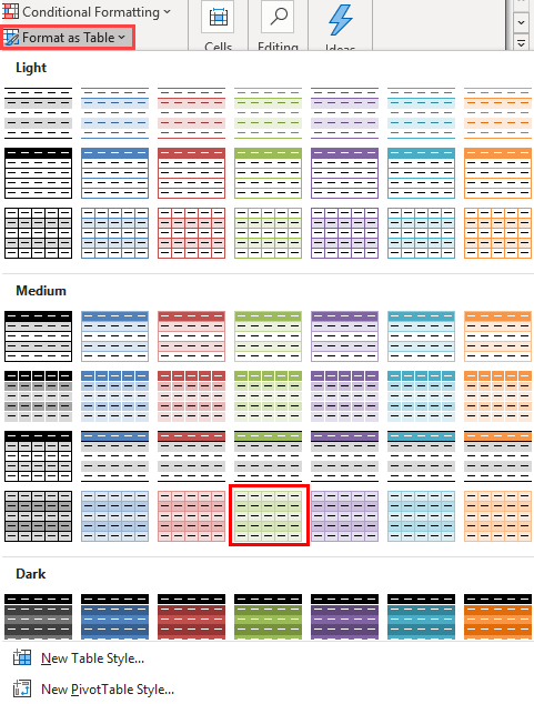
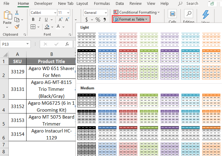
The formatting tables in Let’ssoft Excel are found in the HOME menu under the STYLES group, shown below.
Once we click on the format table, we can find various table styles with alternate row colors, shown below.
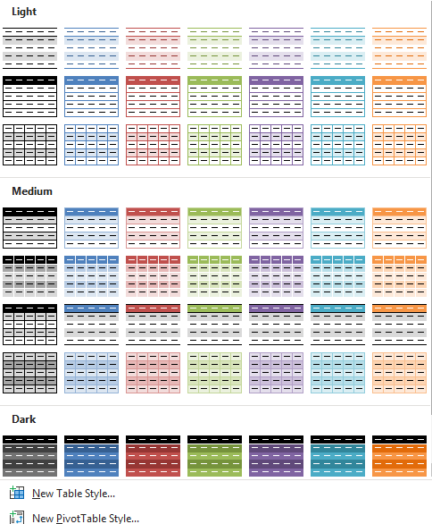
The above screenshot shows that various table styles come with the option like Light, Medium, and Dark.
For example, if we wish to apply a different color to the row, we can simply click the format table and choose any one of the colors that we need to apply.
Example #2 – Applying Alternate Color to the Rows
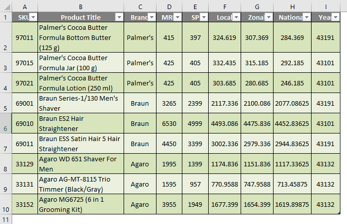
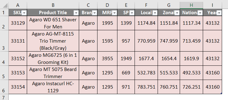
In this example, we will learn how to apply alternate colors to the row using the data below. Consider the below example where we have some sales data tables with no fill color.
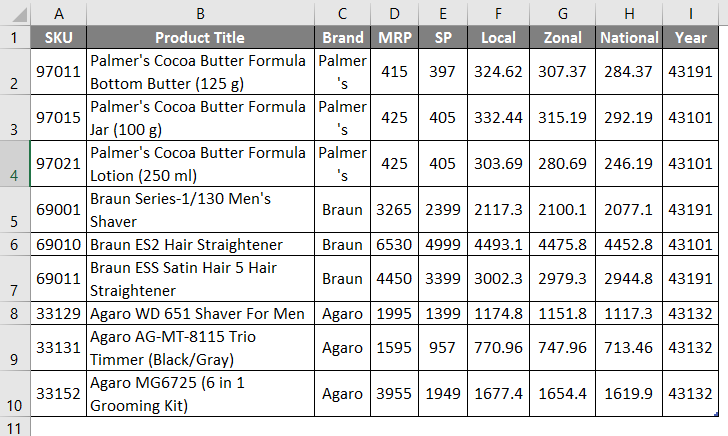
Assume that we must apply alternate colors to the row, making the data more colorful.
We can apply alternate colors to the rows by following the below steps as follows:
First, go to the format table option in the Styles group. Click on the format as table down arrow to get various table styles, as shown below.
Select the row table color to fill it.
Here in this example, we will choose “TABEL STYLE MEDIUM 25”, which shows a combination of dark and light green shown in the screenshot be”ow.
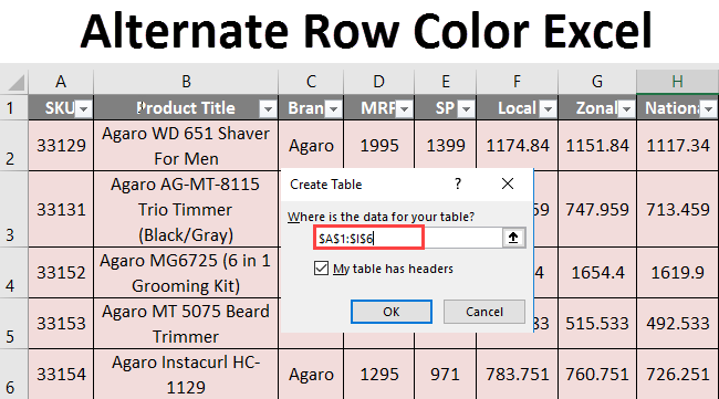
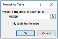
Once we click on “hat MEDIUM table style, we will get the below format table dialog box which is shown below.
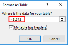
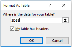
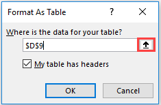
Now, checkmark the “My table HAS HEADERS” because our sales data already had SKU headers, Product title, etc. Next” we need to select t”e range selection for the table. Click on the red arrow mark as shown below.
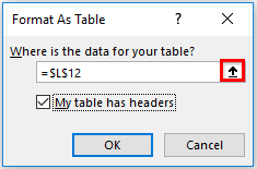
Once we click the red arrow, we will get the selection range below.
Result
We can see that each row has been filled with different alternate row colors in the below result, making the data a perfect view.
Example #3 – Applying Alternate Row Colors using Banding
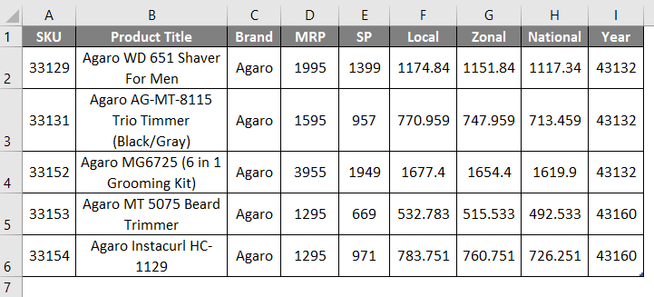
In Microsoft Excel, applying alternate colors is also called Banding, where we have the option while doing table formatting. In this example, we will see how to apply alternate colors to rows using Banding by following the below steps. Consider the below example, which has sales data without formatting.
Now we can apply the banding option using the format table by following the steps below. First, go to the format table option in the Styles group. Click on the format as table down arrow so that we will get the various table styles which are shown below.
Select the row table color to fill it.
Here in this example, we will choose “TABEL STYLE – MEDIUM 24”, which shows a combination of dark and light green shown in the screenshot “elow.
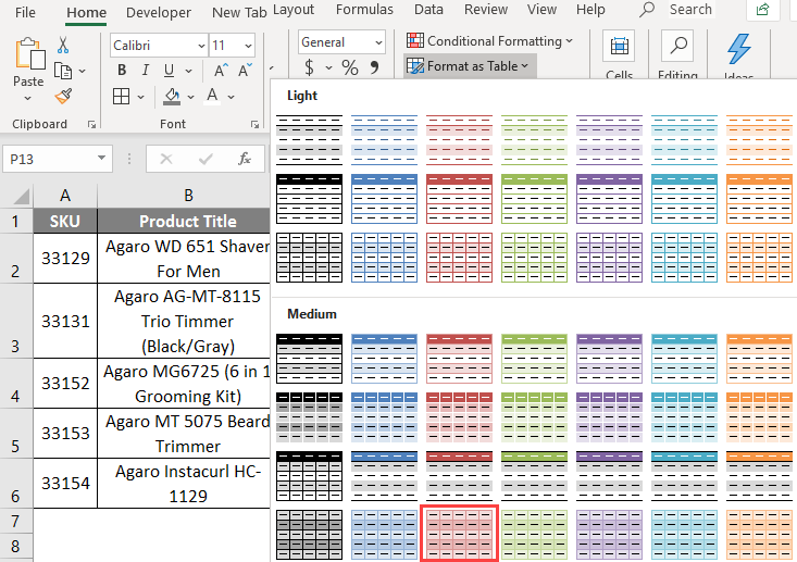
Once we click on “hat MEDIUM table style, we will get the below format table dialog box which is shown below.
Now, checkmark the “My table has headers” because our sales data already has headers named SKU, Product title, etc.
Next” we need to select t”e range selection for the table. Click on the red arrow mark as shown below.
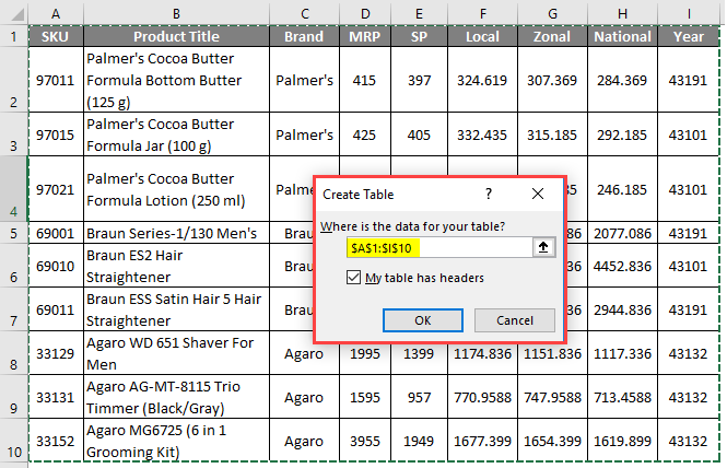
Once we click the red arrow, we will get the selection range below. Select the table range from A1 to I6, shown in the screenshot below.
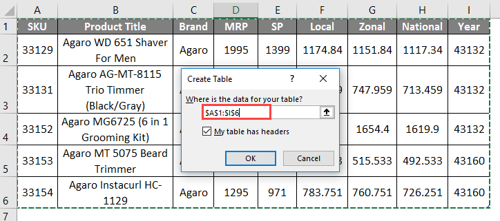
After selecting the range for the table, make sure that “My table has the header” is enabled. Click Ok so that we will get the below result as follows.
Now w” can see that each row “as been filled with alternate colors. We can make the row shading by enabling the option called Banding Rows following the steps below. Select the above-formatted table so that we will get the design menu shown in the screenshot below.
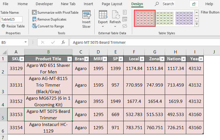
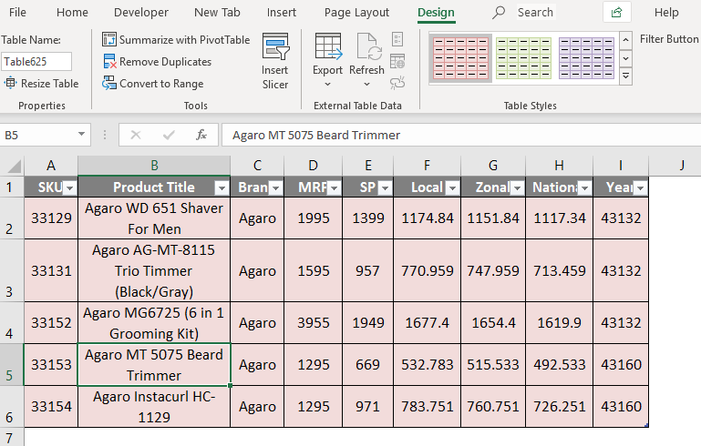
In the design menu, we can notice that “Banded Row” is already enabled, so we are getting the shaded row color. We can disable the Banded ro” by removi”g the checkmark shown in the screenshot below. Once we remove the checkmark for Banded rows, the dark pink color will be removed, shown below.
Results
In the below result, we can notice that the row color has been changed to light pink because of the removal of Banded Rows.
Example #4 – Applying Alternate Row Color using Conditional Formatting
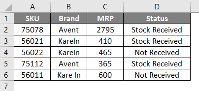
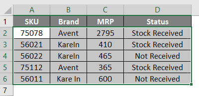
In this example, we will see how to apply alternate row colors using conditional formatting. Consider the below example, which has raw sales data with no row color, which is shown below.
We can apply conditional formatting to display alternate row colors by following the below step. First, select the Brand row to use the Alternate color for the rows shown in the screenshot below.
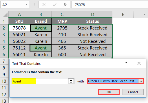
Next, go to conditional formatting and choose “Highlight Cells Rules”, where we will get an option called “Text That Contains”, which is shown belo”.
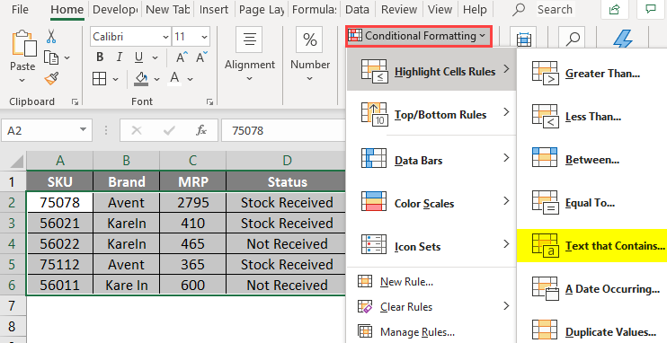
Click the “TEXT” THAT CONTAIN” option to get the dialo” box below.
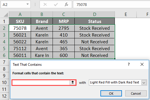
Now in”the dialog box, give the text name on “the right-hand side”, and we can see the drop-down box on the left-hand side where we can choose text color for highlighting. In this example, give the text name Avent and choose the “Green fill with Dark Green Text” shown below.
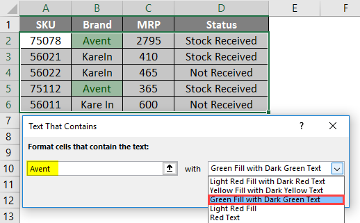
Once we select the Highlight text color, click on Ok
O”ce we click on ok will get the “elow output as follows.
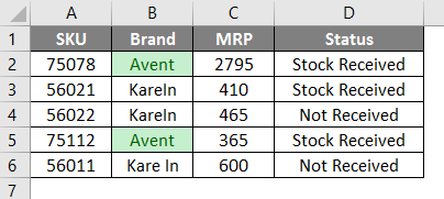
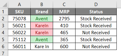
Apply the same for other brand names to get the final output below.
Result
In the below result, we can see that alternate row color has been applied using conditional formatting.
Things to Remember About Alternate Row Color Excel
- We can apply an alternate row color only to the preset tables by formatting the table or using conditional formatting.
- While formatting the table, ensure the header is enabled, or else Excel will overwrite the mentioned headers.
Recommended Articles
This is a guide to Alternate Row Color Excel. Here we have discussed How to add Alternate Row Color Excel, practical examples, and a downloadable Excel template. You can also go through our other suggested articles –
