Updated August 21, 2023
Introduction to REPLACE Formula in Excel
In this article, we will learn about REPLACE Formula in Excel. Normally while working with Excel, we may use the wrong word and want to replace it with the correct word, or sometimes similar pattern data like a month, year, etc., need to update with the new data.
E.g., Where ever Jan is available, we need to replace it with Feb.
The function that helps us to replace the old text with new text without erasing the existing text is called the REPLACE Function. The text may be a single character or a set of characters.
Replace can be performed in two ways:
- With the help of Find and Replace.
- With the use of the Replace Function.
If we press Ctrl + F, we will get the below pop-up.
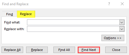
In “Find what,” we need to give the existing text in “Find what,” and in “Replace with,” we need to give the new text. We can replace it in one single cell or all the selected cells in a single click.
Replacement using REPLACE Function:
Another way of replacing is by using the “Replace” function. Replace is a worksheet function that can be used in VBA too.
Syntax:
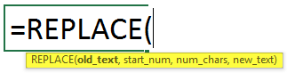
Before seeing a few examples of REPLACE function, we will first understand the 4 arguments that should be input while using the REPLACE function.
An argument in REPLACE Formula:
- Old_text: This argument represents the existing old text.
- Start_num: This argument represents the starting character number from where we want to replace it.
- Num_chars: This argument represents the number of characters we want to replace.
- New_text: This argument represents the new text we want to replace in the old existing text.
How to use Excel REPLACE Formula in Excel?
Excel REPLACE Formula is very simple and easy.
Let’s see how to use the Excel REPLACE Formula with a few examples.
Example #1 – Replace the Text or String
Consider a text string like the one below.
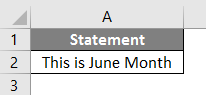
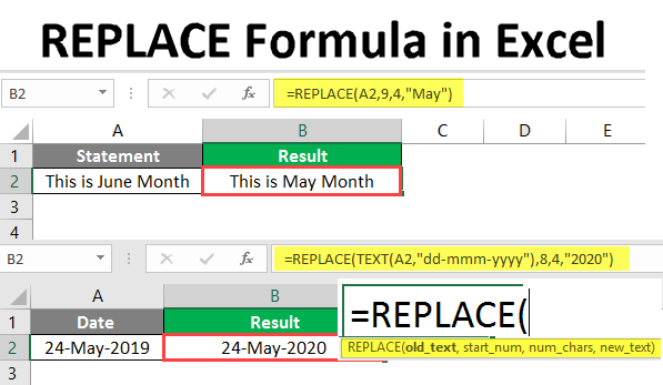
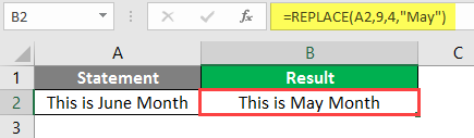
Now we need to replace June with May by using the REPLACE function. Follow the below steps to REPLACE.
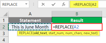
First, select the cell where we want to place the revised text, start the formula, and select the cell with old data. Here A2 is the cell address of existing or old data; hence we selected cell A2.
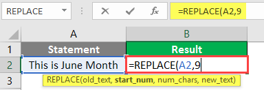
We need to give the start number from which character we want to replace. Here we want to replace E, which is in position number 9. So, give a comma after A2 and input 9.
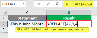
Here “June” occupies 4 characters which we want to replace with new text. How many characters do we want to replace. Input 4 in num_chars position.
The last step is for new text. Input the new text in double quotes, as shown in the below picture.
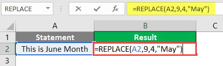
Press Enter Key.
Example #2 – Replace Date with the help of REPLACE Formula
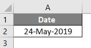
Now we will apply the Replace function to replace a month in date format. Consider a date in the below format.
Now we want to replace 2019 with 2020 using REPLACE. Apply the formula we already applied earlier.
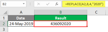
But we got some strange results here. Why? Because the date will save in number format hence, it added 2020 to that number. What is the solution, then?
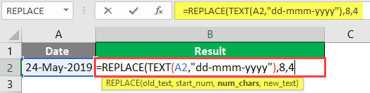
First, we need to convert the data into text format using the TEXT function, and the format is “dd-mmm-yyyy” Then, we will replace 2019 with 2020.
In “Old text”, use the TEXT function to convert the date into the required date format as below.
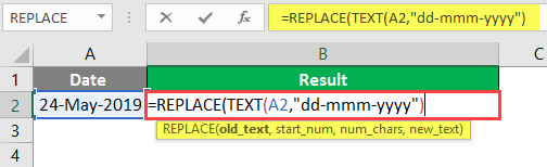
With the above step, we converted the date in cell G11 into text format “dd-mmm-yyy”, and now we can input the rest of the arguments as usual.
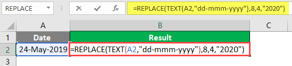
We want to replace 2019 with 2020 hence input 8 in “start_numb” as the 2 is in the 8th position of the string.

Input the number of characters as 4 because “2019” occupies 4 characters.
Finally, input the new text “2020” in double quotes.
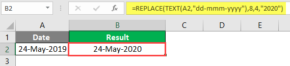
Press Enter Key.
Example #3 – Insert Characters and NESTED REPLACE
In this example, we will see how to input additional characters or symbols without replacing any text and how to use multiple replace conditions.
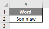
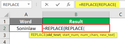
Consider a string “son-in-law” without a symbol “-“as below.
As usual, start the formula REPLACE but don’t select the cell address immediately; instead, input REPLACE function one more time as below.
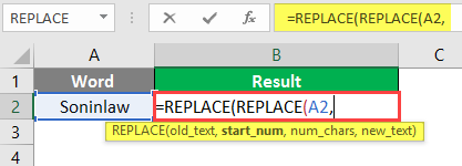
Select the cell address.
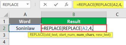
In the start number, input 4 because we need a hyphen character in the fourth position.
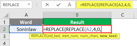
Input zero instead of the number of characters; we do not want to replace any characters here.
Input Hyphen Symbol (-) instead of new text with double quotes.
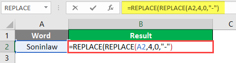
With this, we can input the first hyphen symbol between “son” and “in”, and the result of this replace function will be input for the outer replace function.
Again, input the start number as 7, the number of characters as 0, and the new text as a hyphen as below.
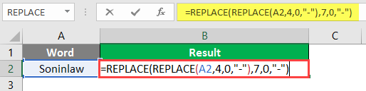
The result will be as below.
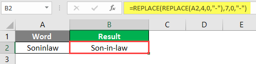
In the above example, we did not remove any characters from the existing or old text but added an additional symbol. Not only symbols but we can also add the characters. Here we used two REPLACE functions; however, we can add multiple REPLACE functions per our requirement.
Things to Remember about REPLACE Formula in Excel
- It is used to replace the old text with new text when we know the position of the text.
- If you do not know the position of old text, you better avoid using it or use it with the FIND function. In the start_num position, use the FIND function.
- If you do not want to remove any character, input zero in the number of characters.
- While working with Dates, ensure you convert it into text and later replace it with the required text. If the result requires in Date format, not in text format, then input the DATEVALUE function to the result of REPLACE function.
Recommended Articles
This has been a guide to REPLACE Formula in Excel. Here we discussed how to use the REPLACE formula in Excel, practical examples, and a downloadable Excel template. You can also go through our other suggested articles to learn more –
