Updated September 30, 2023
![]()
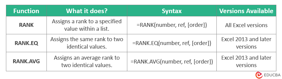
RANK in Excel
The RANK function in Excel shows where a number stands in a list. It helps identify if the number is the highest, lowest, or in between. For example, if students’ scores are 89, 96, and 78 in an exam, you can rank them as 2nd, 1st, and 3rd using RANK in Excel.
Here’s the basic syntax for RANK in Excel:
![]()
This syntax includes two mandatory and one optional argument:
- number: This is the value or number you want to find the rank for.
- ref: This is the range of numbers you want to compare your “number” to.
- [order] (optional): This indicates the ranking order as follows:
1 means ascending (the lowest value gets rank 1).
Types
In Excel, you can use three rank functions:
- RANK
- RANK.EQ
- RANK.AVG
If you start typing “rank” in Excel, it displays all three options.
![]()
You can choose the rank in Excel function that fits your needs best. Here’s what each rank function in Excel does:
How to Use the RANK Function in Excel?
Let’s understand how to use rank in Excel through practical examples. We have covered each type for a clear understanding.
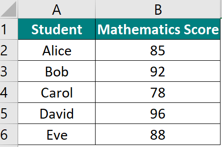
Example #1: RANK Function (For Different Values)
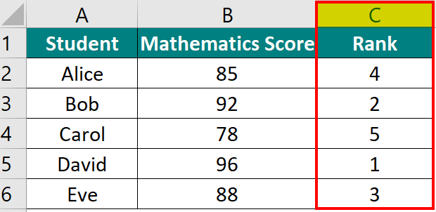
Consider a list of students’ scores in a Math exam. We want to rank the student with the highest score as 1, and so on, based on their rankings.
Solution:
Step 1:
- In a new column (Column C), type this formula in cell C2:
=RANK(B2, $B$2:$B$6, 0)
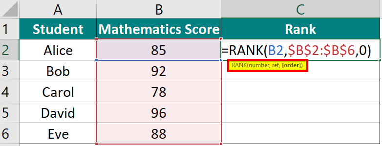
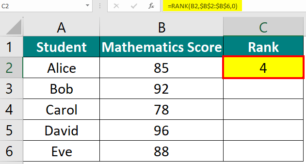
Step 2:
- Press Enter after typing the formula.
- It shows Alice’s rank as 4.
Step 3:
- Select cell C2, then drag the small square that you see at its bottom right corner downwards.
- Column C will now show all rankings.
As you can see in the image below, David, with a score of 96, ranks 1, and Carol, scoring 78, ranks 5.
Note: The formula breakdown is as follows:
- B2: Represents the first student’s score (e.g., Alice’s score).
- $B$2:$B$6: It is the range holding all scores. We have used absolute references to lock this range when copying the formula.
- 0: indicates that we want to rank in descending order (the highest score will get rank 1).
Example #2: RANK Function (For Identical Values)
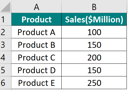
Now, we have a sales dataset where two products, Product B and Product D, show the same sales value of $150 Million. Let’s rank these products accordingly.
Note: We will use “0” as the 3rd argument in the formula. Therefore, excel will rank in descending order.
Given:
1. In cell C2, type this formula:
=RANK(B2, $B$2:$B$6, 0)
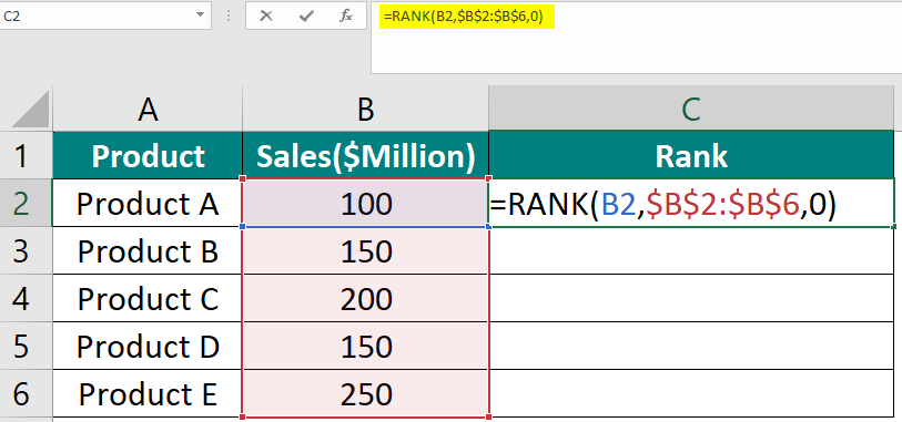
2. When you press Enter, Excel will show the rank as 5 for the first product.
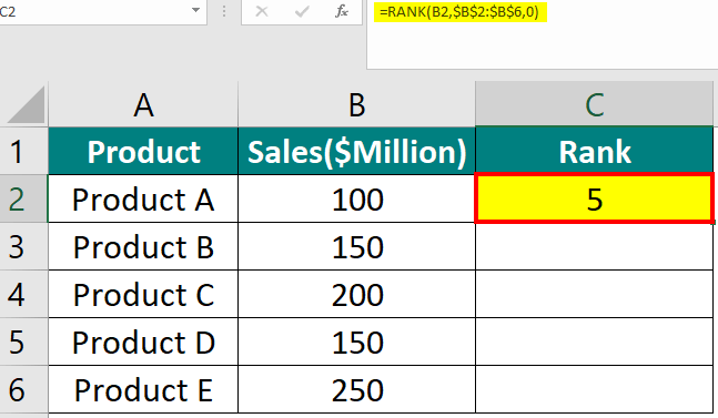
3. Drag the fill handle to extend the formula for the other products. The rank for each product will be displayed as follows.
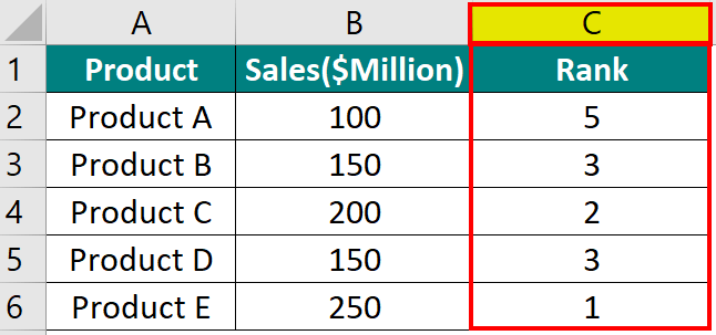
Why there isn’t a 4th rank?
Excel doesn’t assign a 4th rank due to the tie between the sales value of Product B, and Product D. Excel assigns them both rank 3 and skips rank 4.
So, in this case:
- Products B and D share the 3rd rank.
- Product A gets the 5th rank.
Example #3: RANK.EQ Function (For Identical Values)
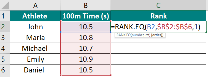
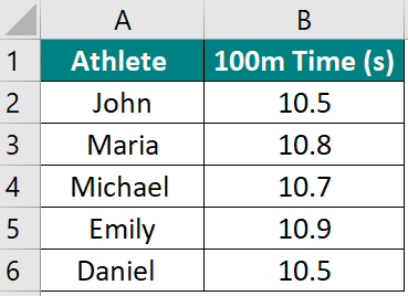
We have a dataset for a race where two athletes, John and Daniel, finish in 10.5 seconds. Let’s rank them using the RANK.EQ function in Excel.
Note: We will use “1” as the 3rd argument in the formula. Therefore, excel will rank in ascending order.
Given:

Solution:
1. In cell D2, type the formula:
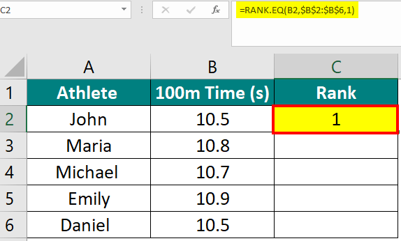
=RANK.EQ(B2,$B$2:$B$6,1)
2. After pressing Enter, Excel calculates John’s rank as 1.
3. Copy the formula to other cells to apply it to all athletes in the list.
Ranks for all athletes will be as follows:
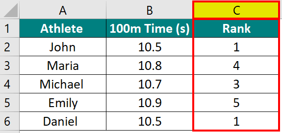
Result:
- John and Daniel share the same time (10.5 seconds); therefore, both get rank 1.
- Michael is ranked 3 because Excel skips rank 2 due to the tie between John and Daniel.
Example #4: RANK.AVG Function (For Different Values)
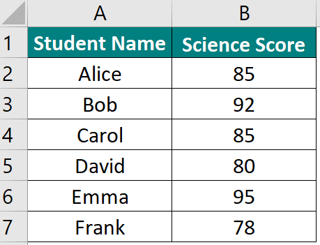
We have a list of student names and their science exam scores. Let’s use the RANK.AVG function to rank these students based on their scores.
Given:

- In cell C2, enter the following formula:
=RANK.AVG(B2,$B$2:$B$7,0) - Press Enter. Excel will calculate the rank for Alice as 5.
- Copy the formula in column C to rank the other students.
![]()
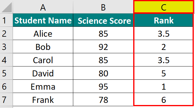
Ranks for all students will be as follows:
Result:
- Emma has the highest score of 95 and gets rank 1.
- Bob has the second-highest score of 92 and gets rank 2.
- Both Alice and Carol scored 85. RANK.AVG recognizes this tie and assigns them an average rank of 3.5.
- David has a score of 80 and gets rank 5.
- Frank has the lowest score of 78 and gets rank 6.
Advanced Applications of RANK Functions
1. RANK + COUNTIF Function
Criteria 1: To rank in descending order
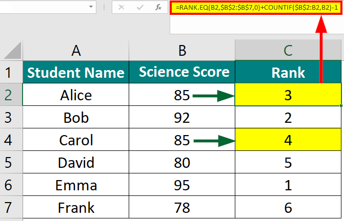
Alice and Carol scored 85 in the Science exam. We want to assign them unique ranks, meaning they should have different ranks. We will use RANK and COUNTIF functions to do this. Also, we will rank the scores in descending order (the highest score will receive rank 1).
Given:
Solution:
- Type this formula in cell C2: =RANK.EQ(B2,$B$2:$B$7,0)+COUNTIF($B$2:B2,B2)-1
- Press Enter after typing the formula. It shows Alice’s rank as
- Apply the formula to all other cells by dragging it down.
- Column C will now show the unique rank values.
Result:
Here’s how unique ranks are decided for the same score:
- The ranking depends on the order in which individuals are listed.
- For instance, Alice, listed before Carol, gets a higher rank (3rd) than Carol (4th).
Note: The formula works like this:
- EQ(B2,$B$2:$B$7): Determines B2’s position in column B.
- COUNTIF($B$2:B2, B2): Counts how many times B2 appears in the list up to the current row.
- Subtracting 1: Prevents rank skips for duplicate values. It means that each value gets a distinct rank.
Criteria 2: To rank in ascending order
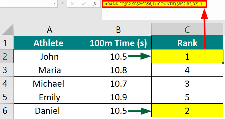
John and Daniel both finished a 100m race in 10.5 seconds. We want to assign them unique ranks. Also, we will rank all the athletes in ascending order (the lowest time will receive rank 1).
Given:
- Type the following formula in cell C2: =RANK.EQ(B2,$B$2:$B$6,1)+COUNTIF($B$2:B2,B2)-1.
- Follow the same process as the previous example (steps 2, 3, and 4).
Result:
2. RANK.EQ + COUNTIFS Function
Criteria: Rank in Excel based on Multiple Criteria
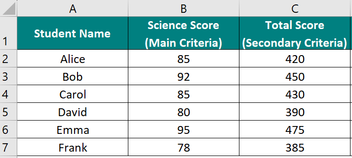
In this example, we have a list of students with their Science Scores (Main Criteria) in column B and Total Scores (Secondary Criteria) in column C. Alice and Carol’s Science Score is the same (85). However, their total scores differ (420 and 430, respectively). To handle this, we will use a combination of RANK.EQ function and COUNTIFS function to rank them fairly.
Given:
Solution:
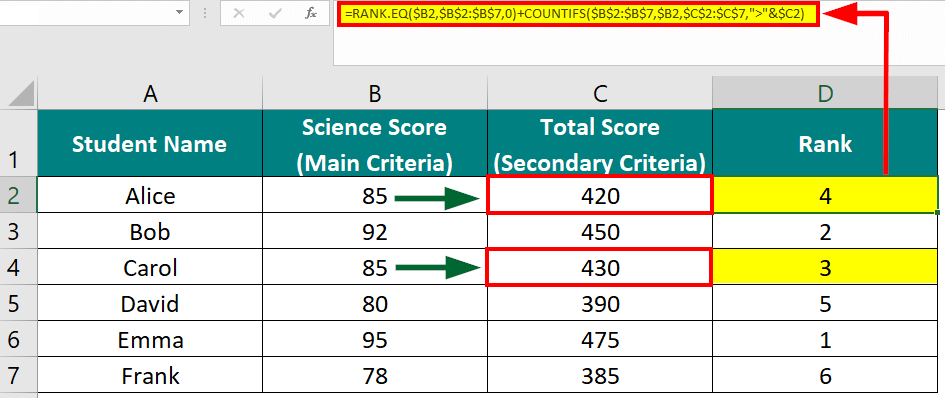
- Enter this formula in cell D2:
RANK.EQ($B2, $B$2:$B$7, 0) + COUNTIFS($B$2:$B$7, $B2, $C$2:$C$7, “>”&$C2) - Press Enter after typing the formula.
- Alice ranks 4th because her Total Score (420) is lower than Carol’s (430).
- Copy and apply the formula to all other cells.
- Column D will now show the rank for multiple criteria.
Result:
This formula considers both Science Scores and Total Scores to determine ranks fairly. If a student excels in both categories (like Carol), they receive a better rank (3rd rank) compared to another student (Alice – 4th rank).
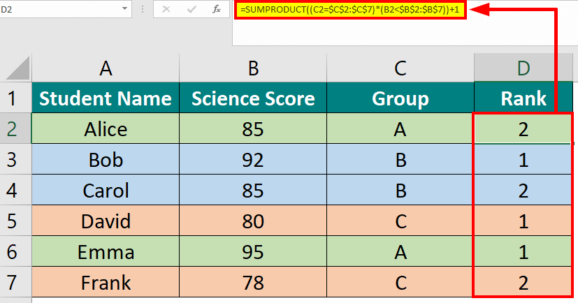
3. Rank Based on the Group
Criteria 1: Rank Highest to Lowest
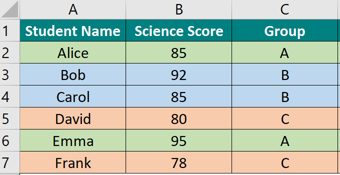
Here, we will assign ranks (highest to lowest) to students within each group using the SUMPRODUCT function.
Given:
Solution:
- Enter this formula in cell D2 and press Enter:
=SUMPRODUCT((C2=$C$2:$C$7)*(B2<$B$2:$B$7))+1
Note: This formula calculates the rank of each student’s science scores within their respective groups.
- Then, copy cell D2 and paste it down for all the rows where you have data (in this case, down to D7).
In column D, you will now have the group rank for each student within their respective groups.
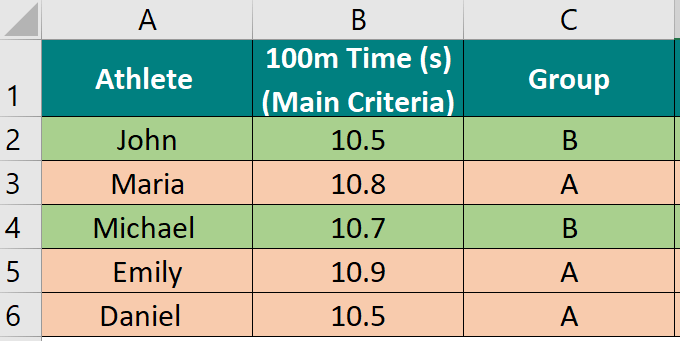
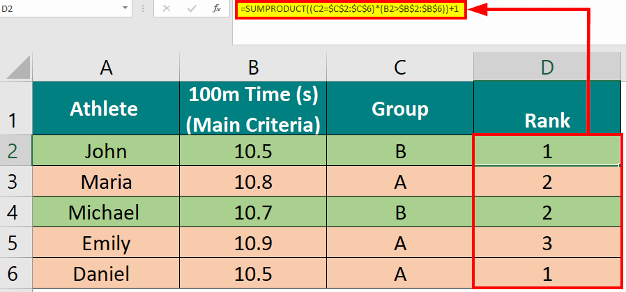
Criteria 2: Rank Lowest to Highest
Here, we will assign ranks (lowest to highest) to athletes within each group using the SUMPRODUCT function.
Given:
Solution:
Use this formula and repeat the same step from above:
=SUMPRODUCT((C2=$C$2:$C$6)*(B2>$B$2:$B$6))+1
Things to Remember
- The RANK function in Excel only accepts numerical values. Using anything else will result in a #VALUE! error.
- If the number you are testing is not in the list, Excel displays a #N/A! error to indicate its absence.
- RANK in Excel gives the same ranking in the case of duplicate values. To get unique ranks for duplicates, use the COUNTIF function.
- The function doesn’t need sorting data in ascending or descending order; it works efficiently regardless of the data’s arrangement.
Recommended Articles
We hope this explanation of RANK in Excel clarifies your queries about this topic. You can also go through our other suggested articles –
