R CSV Files

Introduction to R CSV Files

CSV files are widely used to store the information in tabular format each line being data record. In order to read, write or manipulate data in R, we must have some data available with us. Data can be found on the internet or can be gathered from various sources such as surveys. Using R one can read, write and edit the data which are stored in an external environment. R can read and write data from various formats like XML, CSV, and excel. In this article, we will see how R can be used to read, write and perform different operations on CSV files.

Creating CSV File in R

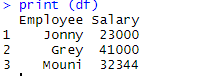
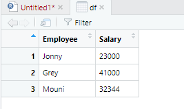
We will see how a data frame can be created and exported to the CSV file in R. In the first, we will create a data frame that consists of variables employee and respective salary.

Code:

> df <- data.frame(Employee = c('Jonny', 'Grey', 'Mouni'),
+                  Salary = c(23000,41000,32344))
> print (df)

Output:

Once the data frame is created it’s time we use R’s export function to create CSV file in R. In order to export the data-frame into CSV we can use the below code.

Code:

> write.csv(df, 'C:\\Users\\Pantar User\\Desktop\\Employee.csv', row.names = FALSE)

In the above line of code, we have provided a path directory for our data fame and stored the dataframe in CSV format. In the above case, the CSV file was saved on my personal desktop. This particular file will be used in our tutorial for performing multiple operations.

Reading CSV Files in R

While performing analytics using R, in many instances we are required to read the data from the CSV file. R is very reliable while reading CSV files. In the above example, we have created the file, which we will use to read using command read.csv.

Below is the example to do so in R:

Code:

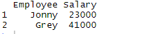
> df <- read.csv(file="C:\\Users\\Pantar User\\Desktop\\Employee.csv", header=TRUE,
sep=",")
> df

Output:

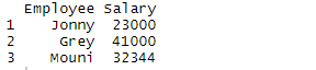
The above command reads the file Employee which is available on desktop and displays that in R studio. Header command implies that the header is made available for the dataset and sep command implies that the data is separated by commas.

Write CSV Files in R

Writing to CSV file is one of the most useful functionalities available in R for a data analyst. This can be used to write an edited CSV file to a new CSV file in order to analyze the data. Write.csv command is used to write the file to CSV.

In the below code df in the data frame in which our data is available, append is used to specify that the new file is created instead of appending or overwriting in the old file. Append false suggests a new CSV file is created. Sep represents the field separated by a comma.

Code:

# Writing CSV file in R
write.csv(df, 'C:\\Users\\Pantar User\\Desktop\\Employee.csv' append = FALSE, sep = “,”)

CSV Operations

CSV operations are required to inspect the data once they have been loaded into the system. R has several built-in functionalities to verify and inspect the data. These operations provide complete information regarding the dataset.

One of the most commonly used command is a summary.

Code:

> summary(df)

Output:

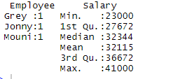
The summary command provides us with column-wise statistics. The numerical variable is described in a statistical way which includes statistical results such as mean, min, median, and max. In the above example, two variables which are Employee and Salary are segregated and statistics for the numerical variable which is Salary is shown to us.

View() command is used to open the dataset in another tab and verify it manually.

Code:

> View(df)

Output:

Str function will provide users more details regarding the column of the dataset. In the below example we can see that the Employee variable has Factor as datatype and the Salary variable has int (integer) as the data type.

Code:

> str(df)

Output:

In many instances, we will need to see the total number of rows available in case of the big dataset, for which we can use the nrow() command.

Code:

> # to show the total number of rows in the dataset
> nrow(df)

Output:

In a similar way to display the total number of columns, we can use ncol() command.

Code:

> ncol(df)

Output:

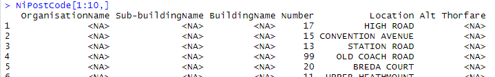
R allows us to display the desired number of rows with the help of below command. When their n number of rows available in the data set, we can specify the range of rows to be displayed.

Code:

> # to display first 2 rows of the data
> df[1:2,]

Output:

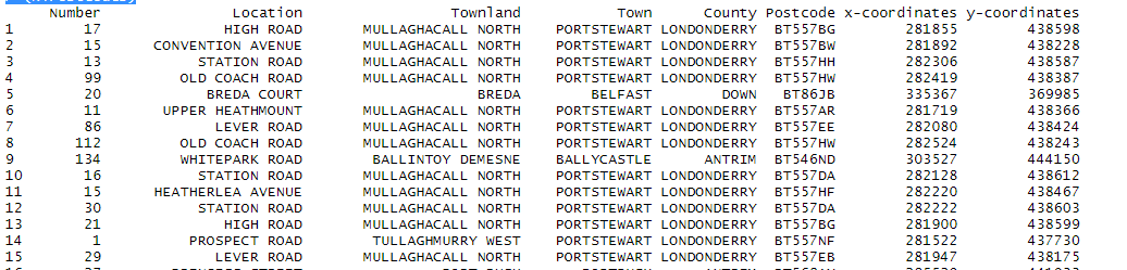
Data operation is performed on the big dataset. For illustration, I’ve downloaded NI postal code open-source dataset from the internet.

Code:

> NiPostCode <- read.csv("NIPostcodes.csv",na.strings="",header=FALSE)

Output:

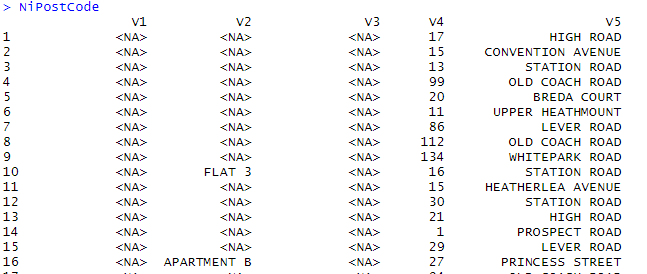
In the above data set, we can see the header names are missing and there many null values present. The dataset requires to be cleaned in order to be made ready for analyzing. In the next step, the headers will be names accordingly.

Code:

> # adding headers/title
> names(NiPostCode)[1] <-"OrganisationName"
> names(NiPostCode)[2] <-"Sub-buildingName"
> names(NiPostCode)[3] <-"BuildingName"
> names(NiPostCode)[4] <-"Number"
> names(NiPostCode)[5] <-"Location"
> names(NiPostCode)[6] <-"Alt Thorfare"
> names(NiPostCode)[7] <-"Secondary Thorfare"
> names(NiPostCode)[8] <-"Locality"
> names(NiPostCode)[9] <-"Townland"
> names(NiPostCode)[10] <-"Town"
> names(NiPostCode)[11] <-"County"
> names(NiPostCode)[12] <-"Postcode"
> names(NiPostCode)[13] <-"x-coordinates"
> names(NiPostCode)[14] <-"y-coordinates"
> names(NiPostCode)[15] <-"Primary Key"

Output:

Now, let’s count the number of missing values in the dataframe and then remove them accordingly.

Code:

> # count of all missing values
> table(is.na (NiPostCode))

Output:

From the above command, we can see the total number of blanks or NA in the dataframe is close to 5445148. Removing all the null values will result in loss of the huge amount of data, hence it’s wise to remove the columns where more than half of 50% of data is missing.

Code:

> # delete columns with more than 50% missing values
> NiPostcodes <- NiPostCode[, -which(colMeans(is.na(NiPostCode)) > 0.5)] > (NiPostcodes)

Output:

Conclusion

In this tutorial, we have seen how CSV files can be created, read and appended using operations in R. We saw how to create a new dataset in R and then import it to CSV format. We have further seen multiple operations such as renaming header and counting the number of rows and columns.

Recommended Articles

This is a guide to R CSV Files. Here we discuss the creating, reading, and writing of CSV file in R with the CSV operations respectively. You may also look at the following article to learn more –

1. JSON vs CSV
2. Data Mining Process
3. Careers in Data Analytics
4. Excel vs CSV