Updated August 11, 2023
QUOTIENT Function in Excel (Table of Contents)
Introduction to Quotient in Excel
Quotient function in Excel comes under the Math and Trig category, which is used for mathematical formulation and returns the integer value with a division of numerator and denominator.
To Quotient, go to Insert function in the Formula menu tab and select Quotient or type equal sign and select this function. Now, as per the syntax, we must have both numerator and denominator in different cells. Select each value that will return the division in the whole number.
Difference between Division Operator and QUOTIENT Function in Excel
In excel commonly we use the division operator forward-slash (/) where this division operator returns the same QUOTIENT when there is a remainder after division number, this divide sign forward-slash(/) returns the decimal number, whereas the QUOTIENT function returns only the integer part and not the decimal number. For example, 1055/190, we will get the output as 5.553, whereas if we use the same number by applying the Quotient function =QUOTIENT (1055, 190), we will get the output as 5.
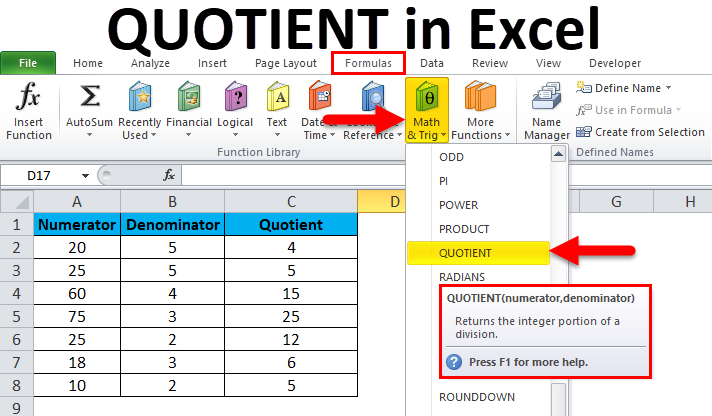
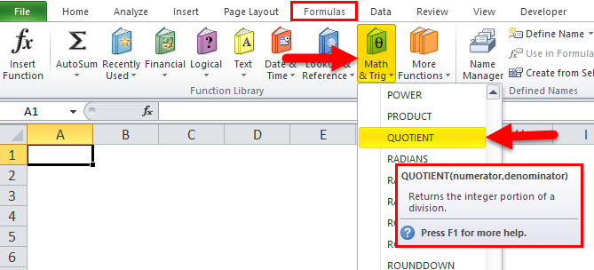
The Microsoft excel QUOTIENT built-in function is categorized under the MATH/ TRIG group, where we can find it under the formula menu shown below.
QUOTIENT Formula in Excel
Below is the QUOTIENT Formula in Excel :
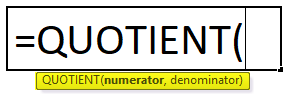
The QUOTIENT formula in excel has two arguments:
- Numerator: This is a dividend with an integer value.
- Denominator: This is a divisor with an integer value.
How to Use QUOTIENT Function in Excel?
QUOTIENT in Excel is very simple and easy to use. Let’s understand the working of it by some QUOTIENT Formula example.
Example #1 – Using the QUOTIENT Function
In this example, we will see how to apply the QUOTIENT function in excel by using simple numbers.
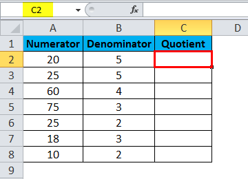
Consider the below example, which shows some random numbers, which are shown below.
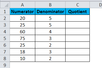
Now we are going to apply the QUOTIENT function in excel by following the below steps.
- First, click on the cell name QUOTIENT on column C2.
- Apply the QUOTIENT formula as shown below =QUOTIENT (A2, B2), where A2 is the numerator and B2 is the denominator.
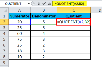
- In the below screenshot, we have selected the columns A2 and B2, which mean A2/B2, which will give the output as 4, which is shown below.
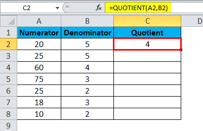
- Drag down the formula to all the cells so that we will get the below output result as follows.
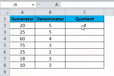
In the above result, we can see that we got the QUOTIENT for the above-mentioned numbers where we can check it manually by applying the forward-slash (/) formula as =A2/B2, which will give us the same output.
Example #2 – Using Division operator (/) and Quotient function
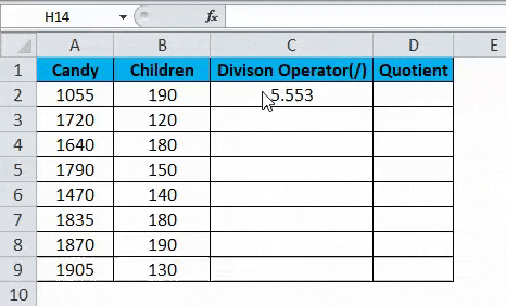
This example shows the difference between the division operator and QUOTIENT function in Excel with the below examples. Consider the below example, which shows a number of candy’s and children where we need to calculate how many candies each child will get.
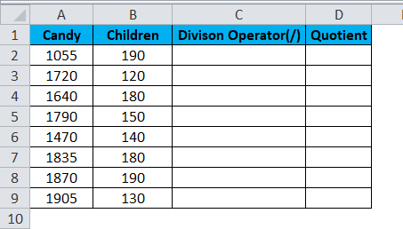
We will use both the division operator and the QUOTIENT function to find out the exact result in excel by following the below result.
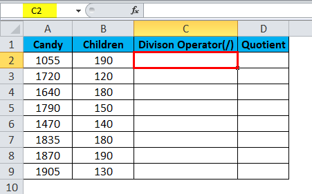
- First, select the cell C2.
- Apply the division formula as =A2/B2.
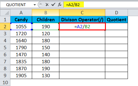
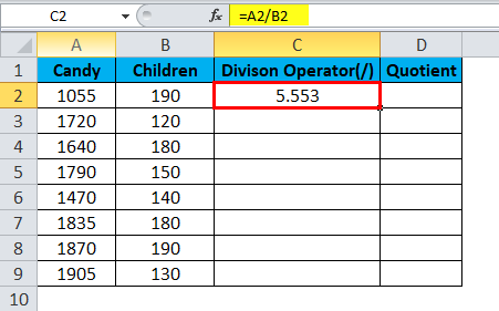
- Here we used the division operator as A2/B2, which means 1055/190, which will give us the output as 5.553 in decimal places, as shown in the below screenshot.
- Now drag down the formula for all the cells so that we will get the output as follows.
Here in the above result, we can see that the division operator calculated the result with decimal places because when there is a remainder after division number, this divide sign forward-slash (/) returns the decimal number where it will create a big confusion that how much candy’s exactly each child will get. To clear this confusion, we can apply the QUOTIENT function in excel by following the below steps.
- First, select the cell D2.
- Apply the QUOTIENT function as =QUOTIENT(A2, B2)
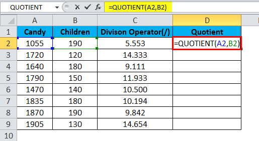
- Here in the above screenshot, we have used Candy as the numerator and Children as the denominator as =QUOTIENT(1055,190), which will give us the output of integer value 5, which is shown below.
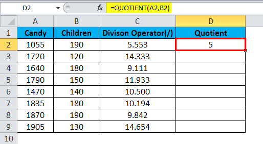
- Now drag down the QUOTIENT formula for all the cells to get the exact output which is shown as a result in the below screenshot.
In the above screenshot, we can see the difference between the division operator, which results in decimal places, whereas the QUOTIENT function returns on the integer value.
Now we can come to the conclusion that each child will get how many candies. For example, let’s take the first figure 1055 candy’s and 190 children; so out of 190 children, each child will get 5 candies with the appropriate result.
Example #3 – Using QUOTIENT Function to return integer portion
In this example, we are going to see how the QUOTIENT function works in excel if we supply any blank value or string in the function.
Let’s consider the below example, which shows random numbers which are shown below.
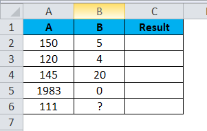
Now we can see that column B contains integer values and also some special characters. Let’s apply the QUOTIENT function in Excel to check the result by following the below steps.
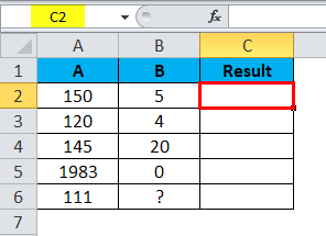
- First, select the cell C2.
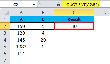
- Apply the QUOTIENT formula as =QUOTIENT(A2, B2).
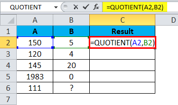
- Here we have applied the QUOTIENT function as 15o as the numerator and 5 as the denominator, which will return the QUOTIENT of 30, which is shown below.
- Now drag down the QUOTIENT formula to all the cells so that we will get the below output as follows.
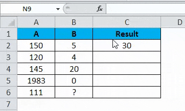
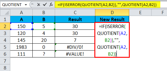
In the above screenshot, we can see that DIV error in column C5 because if the supplied arguments is not an integer value, then the QUOTIENT function will return a DIV error. The same thing happens in the above result because the denominator is zero (0). Next, we can see that we got a VALUE error in C6 Column because the supplied argument is not an integer. It contains special characters that the reason QUOTIENT function has returned VALUE error in the above result.
We can get rid of the above-mentioned errors by using the if statement in QUOTIENT Excel function by applying the below formula:
=IF(ISERROR(QUOTIENT(A2,B2)),””,QUOTIENT(A2,B2))
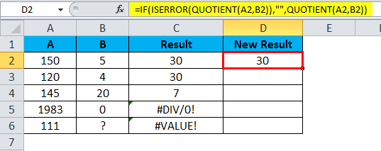
In the above formula, we have applied the if statement along with the ISERROR function, which will check if the value is an error (#N/A, #VALUE,#DIV/0,#NUM) and return TRUE or FALSE.
In the above formula, we have used the QUOTIENT inside the ISERROR, which will check for errors if found any and will return the blank output because we applied double quotes after the QUOTIENT function to return blank output. Hence wherever there is an error, we will get a blank output.
- Now let’s apply the same formula in the above example, which is shown below.
- The result will be as shown below:
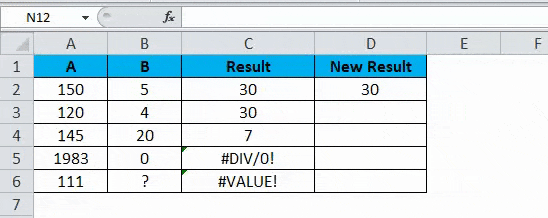
- Now drag down the formula to all the cells so that we will get the below output. In the below result, we can see that we have not received the DIV and VALUE error after applying the formula, which is shown below.
Things to Remember
- QUOTIENT built-in function in excel will return an #DIV/0! Error if the supplied denominator value is blank.
- While using QUOTIENT in Excel, make sure that we are using only integer values.
- In the QUOTIENT Excel function, if the supplied value is not an integer value. i.e. if we apply the string QUOTIENT function, it will throw a #VALUE! Value error.
Recommended Articles
This has been a guide to QUOTIENT in Excel. Here we discuss the QUOTIENT Formula and how to use the QUOTIENT Function in Excel with examples and a downloadable excel template. You may also look at these useful functions in excel –