Updated June 30, 2023
What is Principal Component Analysis
The following article provides an outline for Principal Component Analysis. In data science, we generally have large datasets with multiple features to work on. If the computation of your models gets slow enough or your system is not powerful enough to perform such a huge computation, you might look for alternatives. This is where PCA comes into the picture.
With the help of Principal Component Analysis, you reduce the dimension of the dataset that contains many features or independent variables that are highly correlated with each other while keeping the variation in the dataset up to a maximum extent. The new features created by combining the correlated features are termed principal components. These principal components are the eigenvectors decomposed from a covariance matrix; hence they are orthogonal.

Why do we Need PCA?
PCA is primarily used for dimensionality reduction in domains like facial recognition, computer vision, image compression, and finding patterns in finance, psychology, data mining, etc. PCA extracts important information from the dataset by combining the redundant features. These features are expressed in the form of new variables termed principal components. We can use PCA to reduce the dimensionality of the dataset to 2 or 3 principal components and visualize the results to understand the dataset better. This will be helpful since the features in the dataset have limited visualization.
How Does PCA Work?
The following steps are involved in the working of PCA:
- Data Normalization.
- Computing the Covariance Matrix.
- Computing the Eigen Value and vectors from the Covariance Matrix.
- Choose the first k eigenvectors where k is the required dimension.
- Transform the data points into the k dimension.
1. Data Normalization
It is important to perform data scaling before running PCA on the dataset. Because if we use data of different scales, we get missing leading principle components. To do so, you need to perform mean normalization, and optionally you can also perform feature scaling.
Suppose we have an m dataset, i.e., x1,x2,…..XM of dimension n.
Then compute the mean of each feature using the following equation:
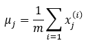
Where,
- uj: It means the jth feature.
- m: Size of the dataset.
- x(i)j: jth feature of data sample i.
Once you have the mean of each feature, then update each x(i)j with x(i)j – uj.
Note that if the features are of a different scale, you must use the following equation to normalize the data.
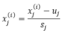
Where,
- x(i)j: jth feature of data sample i.
- sj: The difference between the max and min element of the jth feature.
2. Computing the Covariance Matrix
Assuming that the reader knows about covariance and variance, we will see what the Covariance matrix is represented.
Assuming that we have a dataset of 4 dimensions (a, b, c, d) and the variance is represented as Va, Vb, Vc, Vd for each dimension and covariance is represented as Ca,b for dimensions across a and b, Cb,c for dimension across b and c and so on.
Then the Covariance matrix is given as:
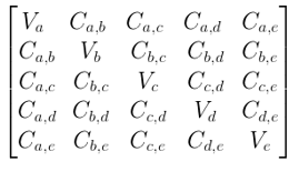
The variance of the dataset is the diagonal element in the Covariance Matrix, while the covariance of the dataset is the off-diagonal element.
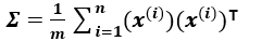
If we have a dataset X of m*n dimension where m is the number of data points, and n is the number of dimensions, then the covariance matrix sigma is given by:
3. Computing the Eigen Value and Vectors from the Covariance Matrix
Now we must decompose the covariance matrix to get the eigenvector and the value. This is done using a single vector decomposition. I won’t be going into the details of svd as it is out of the scope of this article. However, it is important to note that there are functions in popular programming languages like MATLAB, python to compute the svd. You can get the eigenvalue and vector in the octave using the svd() function.
Where,
- Σ: Covariance matrix (Sigma).
- U: Matrix containing the eigenvectors.
- S: Diagonal matrix containing the eigenvalues.
4. Choose the First k Eigenvectors where k is the Required Dimension
Once we have the matrix containing the eigenvectors, we can select the first k columns of it. Where k is the required dimension.
Ureduce is the matrix of the eigenvector that is needed to perform the data compression.
5. Transform the Datapoints into k Dimension
To transform the dataset X n*m from n dimension to k dimension by taking the transpose of the Ureduce matrix and then multiplying it with the dataset.
Where,
- z: Its new features.
- As a result, you will get a dataset of dimension m*k from m*n.
Properties of Principal Component Analysis
Following is the list of properties that PCA possesses:
- It transforms high dimensional data set into a low dimension before using it for training the model.
- Principle components of PCA are the linear combinations of the original features; the eigenvector found from the covariance matrix satisfies the principle of least squares.
- This helps to identify the essential traits that clarify the correlation.
Advantages of Principal Component Analysis
PCA’s main advantage is its low sensitivity towards noise due to dimensionality reduction.
Following are the other advantages of PCA:
- It speeds up the learning algorithm.
- Increases Efficiency due to lower dimensions.
- It reduces the space required to store the data.
- Data visualization.
- Low sensitivity towards the noise.
- Removes redundant variables.
Conclusion
PCA method is a part of the unsupervised machine learning technique. These techniques are most suitable for images that have no class labels. An introduction to PCA and its work has been provided. And as mentioned above, the advantages of PCA have also been discussed in this article.
Recommended Articles
This is a guide to Principal Component Analysis. Here we discuss why we need PCA, how it works with appropriate steps involved, along with the advantages of principal components. You can also go through our other related articles to learn more –