Updated March 24, 2023
Introduction to P-Value in Regression
P-Value is defined as the most important step to accept or reject a null hypothesis. Since it tests the null hypothesis that its coefficient turns out to be zero i.e. for a lower value of the p-value (<0.05) the null hypothesis can be rejected otherwise null hypothesis will hold. In other words, the predictor that holds a lower p-value is likely to be more meaningful addition to the model as a change in the predictor values are related to the changes of the response variable. It is one of the important steps to reject or accept the null hypothesis.
Before we start with P-value, we must have to decode what hypothesis testing is. Hypothesis testing is a test that suggests that interpretation based out on samples is right for the entire population or not. While doing hypothesis testing we have to specify null and alternative hypotheses beforehand.
Null Hypothesis: Suggests that there is no statistical significance between the two variables in the study which we are doing.
Alternative Hypothesis: Suggests that there is a statistical significance between the two variables.
Let’s understand these concepts with some examples.
Imagine we live in a world where the mean consultation time of the doctor for consulting a patient is 15 minutes or less. This is our initial belief that within 15 minutes doctors are able to take a wise call for the patient problem, hence we can say the average time for consultation is 15 minutes or less.
The null hypothesis and alternative hypothesis are:
Null Hypothesis: The average consultation time by the doctor is 15 minutes or less than that. We assume that the null hypothesis is a statement that is a general belief. Like every common and at the same time feels very natural.
Alternative Hypothesis: The average consultation time by the doctor is more than 15 minutes. We assume the alternative hypothesis as the statement which discards the initial belief.
Normal Distribution
Now we will discuss the normal distribution (also known as Gaussian distribution). This distribution is used to see the data distribution. Sometimes the researcher mentioned it as the probability density function also.
Features of Normal Distribution
- It is a part of the central limit theorem
- It produces a bell-shaped curved
- In this distribution Mean = Median = Mode
- Half of the data values are less than 50% and half of the data values are more than 50%
- It has two parameters, one is mean and the other one in Standard deviation
Syntax
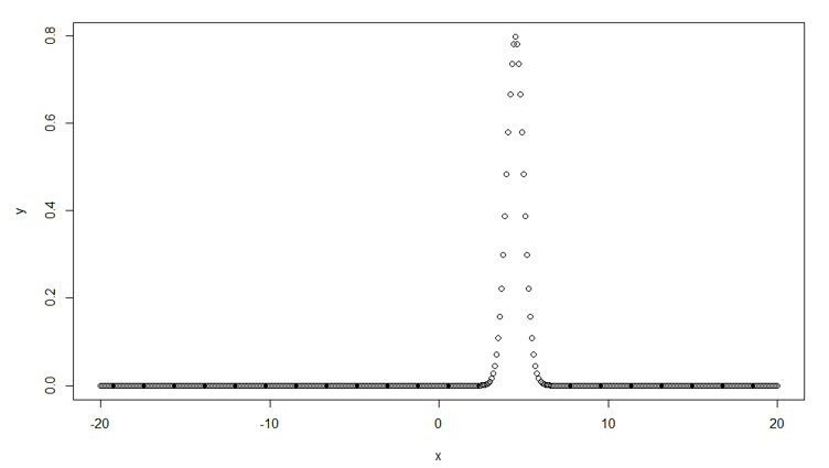
Syntax in R for normal distribution chart looks like:
# Create a sequence of numbers between -20 and 20 incrementing by 0.1.

x <- seq(-20, 20, by = .1)

# Choose the mean as 4.5 and standard deviation as 0.5.

y <- dnorm(x, mean = 4.5, sd = 0.5)

plot(x,y)
Where x is a vector of numbers. The mean value is the mean of the sample which we derive from a population.
Standard deviation is the amount of variation between the set of values and the mean
Significant Level
A significant level tells us that x% is the probability of rejecting the null hypothesis when it is actually true. Here we meant to say that we will reject the null hypothesis which states that the average time of consultation is 15 minutes or less and for real the consultation is time is less than or equal to 15 minutes, and still we reject it. The significant level is also known as “alpha” and denoted as “α”.
P-Value in Regression
We didn’t discuss on what basis we can accept or reject the null hypothesis, let’s discuss that now.
To accept or reject the null hypothesis, we have to consider the P-value of the model. The model here can be regression analysis. Now, we will discuss how to calculate the P-value of a regression model and how to interpret it.
1. Dataset
We will use the “USArrest” dataset here, which is available in Rstudio.
| Murder arrests (per 100,000) | Assault arrests (per 100,000) | Percent urban population | Rape arrests (per 100,000) | |
| Alabama | 13.2 | 236 | 58 | 21.2 |
| Alaska | 10 | 263 | 48 | 44.5 |
| Arizona | 8.1 | 294 | 80 | 31 |
| Arkansas | 8.8 | 190 | 50 | 19.5 |
| California | 9 | 276 | 91 | 40.6 |
| Colorado | 7.9 | 204 | 78 | 38.7 |
| Connecticut | 3.3 | 110 | 77 | 11.1 |
| Delaware | 5.9 | 238 | 72 | 15.8 |
| Florida | 15.4 | 335 | 80 | 31.9 |
| Georgia | 17.4 | 211 | 60 | 25.8 |
| Hawaii | 5.3 | 46 | 83 | 20.2 |
| Idaho | 2.6 | 120 | 54 | 14.2 |
| Illinois | 10.4 | 249 | 83 | 24 |
| Indiana | 7.2 | 113 | 65 | 21 |
| Iowa | 2.2 | 56 | 57 | 11.3 |
| Kansas | 6 | 115 | 66 | 18 |
| Kentucky | 9.7 | 109 | 52 | 16.3 |
| Louisiana | 15.4 | 249 | 66 | 22.2 |
| Maine | 2.1 | 83 | 51 | 7.8 |
| Maryland | 11.3 | 300 | 67 | 27.8 |
| Massachusetts | 4.4 | 149 | 85 | 16.3 |
| Michigan | 12.1 | 255 | 74 | 35.1 |
| Minnesota | 2.7 | 72 | 66 | 14.9 |
| Mississippi | 16.1 | 259 | 44 | 17.1 |
| Missouri | 9 | 178 | 70 | 28.2 |
| Montana | 6 | 109 | 53 | 16.4 |
| Nebraska | 4.3 | 102 | 62 | 16.5 |
| Nevada | 12.2 | 252 | 81 | 46 |
| New Hampshire | 2.1 | 57 | 56 | 9.5 |
| New Jersey | 7.4 | 159 | 89 | 18.8 |
| New Mexico | 11.4 | 285 | 70 | 32.1 |
| New York | 11.1 | 254 | 86 | 26.1 |
| North Carolina | 13 | 337 | 45 | 16.1 |
| North Dakota | 0.8 | 45 | 44 | 7.3 |
| Ohio | 7.3 | 120 | 75 | 21.4 |
| Oklahoma | 6.6 | 151 | 68 | 20 |
| Oregon | 4.9 | 159 | 67 | 29.3 |
| Pennsylvania | 6.3 | 106 | 72 | 14.9 |
| Rhode Island | 3.4 | 174 | 87 | 8.3 |
| South Carolina | 14.4 | 279 | 48 | 22.5 |
| South Dakota | 3.8 | 86 | 45 | 12.8 |
| Tennessee | 13.2 | 188 | 59 | 26.9 |
| Texas | 12.7 | 201 | 80 | 25.5 |
| Utah | 3.2 | 120 | 80 | 22.9 |
| Vermont | 2.2 | 48 | 32 | 11.2 |
| Virginia | 8.5 | 156 | 63 | 20.7 |
| Washington | 4 | 145 | 73 | 26.2 |
| West Virginia | 5.7 | 81 | 39 | 9.3 |
| Wisconsin | 2.6 | 53 | 66 | 10.8 |
| Wyoming | 6.8 | 161 | 60 | 15.6 |
2. Problem
We have to find whether there is a significant relationship between speed and distance in the linear regression model and our significant level is .05
3. Solution
Now we will write the syntax for linear regression.
linear_regression<-lm(Assault ~ UrbanPop, data = USArrests)

print(linear_regression)
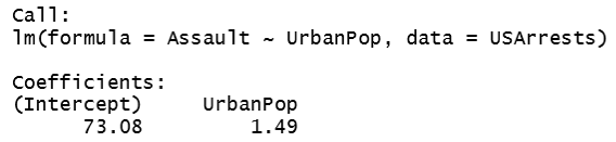
As per the above outcome, our linear regression equation looks like this
Dist = 73.08 + (1.49)Speed
For the summary of the model, we will pass Summary() syntax
linear_regression<-lm(Assault ~ UrbanPop, data = USArrests)

summary(linear_regression)
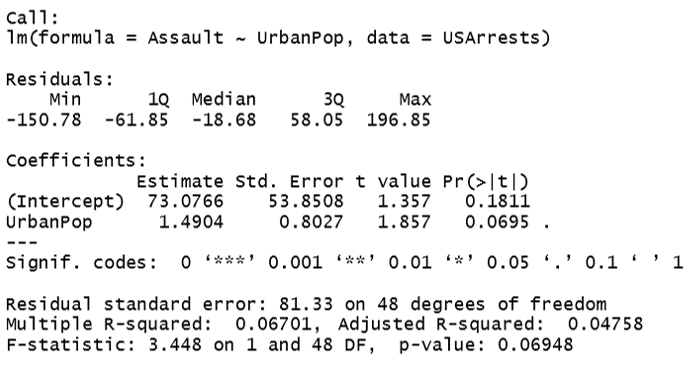
P-value in our model is 0.06948 and it is more than the significant level which is 0.05. Hence, we can conclude that there is no relationship between the “Assault” and the “Urbanpop” variable and we can accept the null hypothesis.
Conclusion
P-value is introduced by Pearson in 1900. It is one of the preferred methods which researchers use to summarize the result of the problems they are dealing with. But taking decisions solely on P-value is not right, it is recommended to consider other contextual factors to derive scientific inferences. Not just P-value, everything from study design, logical assumptions, and quality of measurements are also important.
Recommended Articles
This is a guide to P-Value in Regression. Here we discuss the introduction to P-Value Regression along with the normal distribution, significant level and how to calculate and interpret the P-value of a regression model. You may also look at the following articles to learn more –
